Sentaurus Mesh
2. Using the Axis-Aligned Mesh Generator

2.1 Basics
2.2 Refinement Regions
2.3 Refinement Controls
2.4 Interface Mesh Refinement
2.5 Offsetting
2.6 Multiboxes
2.7 Mesh Smoothing
2.8 Defining the Doping Profile
2.9 Advanced Options

Objectives

• To introduce the axis-aligned mesh generation capabilities of Sentaurus Mesh.

2.1 Basics

Sentaurus Mesh applies axis-aligned mesh generation by default. To run Sentaurus Mesh, use the command:

> snmesh <filename>

Sentaurus Mesh checks the corresponding <filename>_bnd.tdr and <filename>.cmd input files, and then applies the binary-tree discretization to a device domain according to the command file specifications.

The quadtree (2D) or octree (3D) recursive space decomposition technique is used in Sentaurus Mesh to discretize a device domain that is combined with mesh delaunization.

Figure 1 illustrates the concept of quadtree space decomposition for a 2D device. First, the quadrant (called root) is defined, which surrounds the entire device domain (in this case, it exactly matches the device boundary). Second, the recursive split process starts when an entire domain is split by two subdomains in each direction, then, each subdomain is again split by two, and so on, until the domain is resolved according to the mesh control specifications. Third, the entire domain is represented as a union of all leaf elements of the tree, from where it derives its name – the binary tree method.

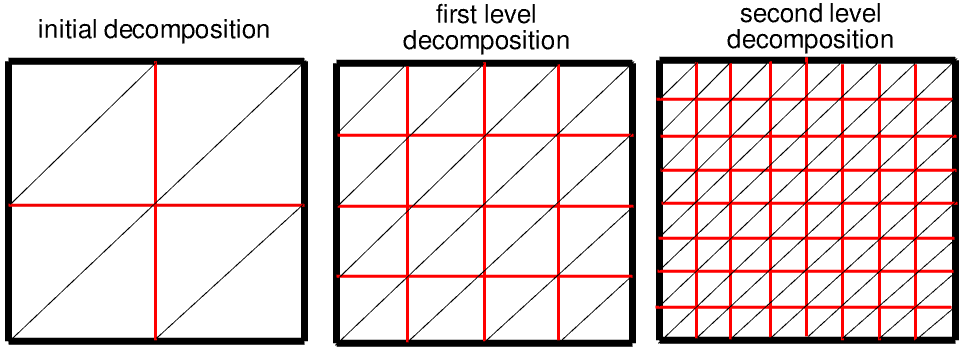
Figure 1. Illustration of the concept of quadtree space decomposition. (Click image for full-size view.)

Sentaurus Mesh requires that a device boundary file is created, preferably by either Sentaurus Process or Sentaurus Structure Editor.

To mesh a device, you must create a command file where general mesh controls and optional doping specifications are defined. A command file can be created either manually (in a text editor) or using the corresponding Sentaurus Structure Editor functionality (see Section 4. Generating Meshes of the Sentaurus Structure Editor module).

The Sentaurus Mesh command files featured in this section are all contained in the Sentaurus Workbench project Applications_Library/GettingStarted/snmesh/Basics. Within this project, the preferences are selected such that Sentaurus Mesh will take the boundary file from the preceding Sentaurus Structure Editor tool instance, while the command file is created by a text editor (see Section 1.6 Sentaurus Mesh Integration in Sentaurus Workbench).

To work with the project, start Sentaurus Workbench and copy the project Basics to a local directory within your Sentaurus Workbench working directory to which the environment variable $STDB points. For details about this environment variable, see Section 1.2 Starting Sentaurus Workbench.

The features discussed in this section are demonstrated in the Sentaurus Mesh tool instance labeled test2d in this Sentaurus Workbench project.

A command file must include at least two independent sections. In the Definitions section, you specify mesh spacing controls (Refinement) and doping profiles, which then can be referenced in the Placements section.

First, you will mesh a piece of silicon material (2 μm x 2 μm).

Click to view the command file test2d_msh.cmd.

In this command file, only a single Refinement statement called "global" is declared, which specifies the maximum-allowed mesh element size as 0.5 μm in each of the spatial directions of the device. The "global" refinement is referenced in the Placements section under the same name without any position specification, indicating that the entire device will be meshed using the refinement specification in the Definitions section:

Definitions {
  Refinement "global" {
    MaxElementSize = (0.5 0.5)
  }
}
Placements {
  Refinement "global" {
    Reference="global"
  }
}

where the two values in the MaxElementSize specification indicate the maximal mesh step in the x- and y-direction.

For 2D device meshing, the value that corresponds to the third device dimension (usually, the z-coordinate) can be omitted.

Figure 2 shows the mesh generated by Sentaurus Mesh. Run the corresponding project node and view the generated mesh with Sentaurus Visual.

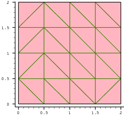
Figure 2. Mesh generated by Sentaurus Mesh.

In Figure 2, you can see that the entire device first is decomposed into 16 rectangles (four in each direction), which then are triangulated. In this case, the edge length of each rectangle is 0.5 μm exactly, as specified in the refinement definition. The final mesh consists of 25 vertices and 32 elements.

For a similar (2 μm x 2 μm x 2 μm) 3D device structure and the command file test3d_msh.cmd, the final mesh consists of 125 vertices and 384 elements as shown in Figure 3.

Click to view the command file test3d_msh.cmd.

Run the project node of Sentaurus Mesh labeled test3d and view the generated mesh with Sentaurus Visual.

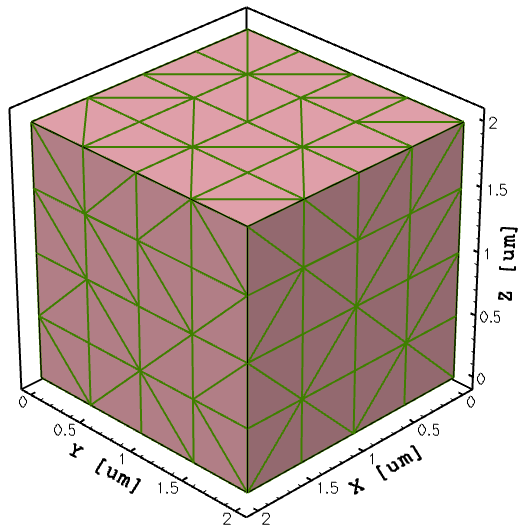
Figure 3. Three-dimensional device with 125 vertices and 384 elements.

Having MaxElementSize control values not strictly proportional to the entire device dimensions results in a smaller element size than specified. For the above 2D device structure, the 0.4 μm maximal step value is specified in each direction:

Definitions {
  Refinement "global" {
    MaxElementSize = (0.4 0.4)
  }
}

With this setting, you can expect to have 2 μm/0.4 μm = 5 mesh steps in each direction. However, the binary-tree decomposition algorithm produces eight (8) steps in each direction (see Figure 4), which results in 128 mesh elements and 81 mesh vertices. This example makes it clear that, in most cases, the resulting mesh step will be lower than specified due to the specifications of the binary-tree decomposition algorithm.

This behavior is exemplified in the project Basics at the Sentaurus Mesh tool instance labeled finerMesh. Run the corresponding project node and view the generated mesh with Sentaurus Visual.

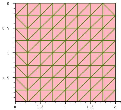
Figure 4. Two-dimensional mesh with smaller mesh steps.

Now, you will see what happens with a nonaxis-aligned device. In this example, the device boundary used in the previous example is rotated 45°, and the same command settings as in the command file of the first example (rot2d_msh.cmd) are applied.

Click to view the command file rot2d_msh.cmd.

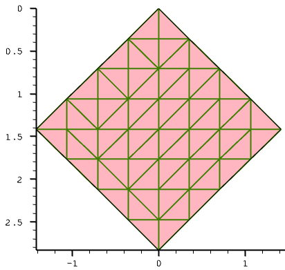
Figure 5. Two-dimensional mesh with smaller mesh steps, which is rotated 45°.

As can be seen in Figure 5, for a rotated (nonaxis-aligned) structure, the binary-tree decomposition is applied to a larger domain, resulting in a larger number of mesh nodes. The final mesh consists of 78 elements and 55 vertices.

This behavior is exemplified in the project Basics at the Sentaurus Mesh tool instance labeled rot2d. Run the corresponding project node and view the generated mesh with Sentaurus Visual.

2.2 Refinement Regions

The Sentaurus Mesh command files featured in this section are all contained in the Sentaurus Workbench project Applications_Library/GettingStarted/snmesh/Refinements.

To work with the project, start Sentaurus Workbench and copy the project Refinements to a local directory within the Sentaurus Workbench working directory to which the environment variable $STDB points. For details about this environment variable, see Section 1.2 Starting Sentaurus Workbench.

As mentioned in Section 2.1 Basics, the refinement region is a geometric object, placed inside a device, which allows flexible control over a mesh step. The refinement region is represented by a geometric element, such as a rectangle, polygon, or complex polygon in the case of two dimensions, or a cuboid or polyhedron (the closed volume surrounded by multiple polygons) in the case of three dimensions. It also can refer to an entire material or region.

The syntax to define a refinement region in the Definitions section of the command file is:

Refinement "reference name" {
  MaxElementSize = (<xmax> <ymax> <zmax>)
  MinElementSize = (<xmin> <ymin> <zmin>)
  RefineFunction = MaxGradient(parameters) | MaxTransDifference(parameters) |
                   MaxLengthInterface(parameters)
}

where:

• MaxElementSize and MinElementSize indicate the maximum-allowed and minimum-allowed mesh step values inside a refinement region along a particular axis.
• RefineFunction specifies the mesh refinement controls (see Section 2.3 Refinement Controls).
• MaxLengthInterface activates mesh refinement at interfaces (see Section 2.4 Interface Mesh Refinement).

The corresponding refinement instance definition in the Placements section is:

Placements {
  Refinement "instance name" {
    Reference = "string"
    RefineWindow = geometric element | material | region
  }
}

For multiple refinement specifications, the refinement regions can overlap. If this is the case, a refinement region with the smallest step definition "wins".

The following example demonstrates this, with the rectangular refinement region inside the test device structure with smaller step definitions compared to the global ones:

Definitions {
  Refinement "global" {
    MaxElementSize = (0.5 0.5 0.5)
  }
  Refinement "rectangle" {
    MaxElementSize = (0.125 0.125 0.125)
  }
}

Placements {
  Refinement "global" {
    Reference="global"
  }
  Refinement "rectangle" {
    Reference = "rectangle"
    RefineWindow = Rectangle [(0.75 0.75) (1.25 1.25)]
  }
}

The resulting mesh is shown in Figure 6, where the contour of the rectangular refinement region is highlighted. The transition from the finer mesh inside the rectangular refinement to the coarser mesh outside the region, due to mesh smoothing, is clearly seen (see Section 2.7 Mesh Smoothing).

This behavior is exemplified in the project Refinements at the Sentaurus Mesh tool instance labeled rectangle. Run the corresponding project node and view the generated mesh with Sentaurus Visual.

Figure 6. Rectangular 2D refinement.

The next example demonstrates the regionwise refinement approach, where the polygonal region called PolygonR is introduced inside the device test structure.

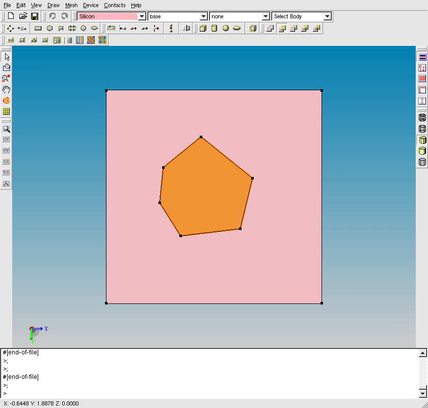
Figure 7. Polygonal region inside device structure shown in Sentaurus Structure Editor. (Click image for full-size view.)

Different refinement criteria are used inside and outside the polygonal region refinement. Inside the polygonal region, a smaller mesh step is specified, compared to the global step definition:

Definitions {
  Refinement "global" {
    MaxElementSize = (0.5 0.5 0.5)
  }
  Refinement "polygon" {
    MaxElementSize = (0.25 0.25 0.25)
  }
}

To confine the mesh refinement inside the polygonal region, the regionwise refinement placement is defined using the RefineWindow specification:

Placements {
  Refinement "global" {
    Reference="global"
  }
  Refinement "polygon" {
    Reference = "polygon"
    RefineWindow = region ["PolygonR"]
  }
}

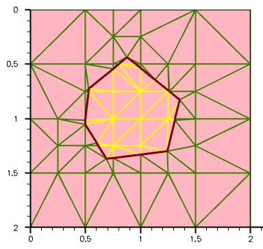
Figure 8. Polygonal mesh refinement.

This behavior is exemplified in the project Refinements at the Sentaurus Mesh tool instance labeled polygon. Run the corresponding project node and view the generated mesh with Sentaurus Visual.

Different mesh colors help to visualize the transition from denser to coarser mesh areas.

The next example demonstrates how materialwise mesh refinement is performed. In this example, two adjacent materials, silicon and oxide, are meshed with different mesh steps (0.5 μm in silicon and 0.125 μm in oxide):

Definitions {
  Refinement "Si" {
    MaxElementSize = (0.5 0.5 0.5)
  }
  Refinement "Ox" {
    MaxElementSize = (0.125 0.125 0.125)
  }
}

Placements {
  Refinement "Si" {
    Reference = "Si"
    RefineWindow = material ["Silicon"]
  }
  Refinement "Ox" {
    Reference = "Ox"
    RefineWindow = material ["Oxide"]
  }
}

Figure 9 shows the resulting mesh. The smaller mesh step propagates from the silicon–oxide material interface towards silicon because of the applied mesh smoothing (see Section 2.7 Mesh Smoothing).

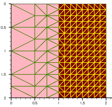
Figure 9. Materialwise mesh refinement.

This behavior is exemplified in the project Refinements at the Sentaurus Mesh tool instance labeled materials. Run the corresponding project node and view the generated mesh with Sentaurus Visual.

2.3 Refinement Controls

One of the major features of Sentaurus Mesh is automatic mesh refinement, which allows you to accurately resolve areas with geometry or profile spatial nonuniformities. This section discusses the mesh refinement of a nonuniform doping distribution.

The Sentaurus Mesh command files featured in this section are all contained in the Sentaurus Workbench project Applications_Library/GettingStarted/snmesh/RefineControls.

To work with the project, start Sentaurus Workbench and copy the project RefineControls to a local directory. The target directory must reside under the Sentaurus Workbench working directory to which the environment variable $STDB points. For details about this environment variable, see Section 1.2 Starting Sentaurus Workbench.

The following example demonstrates automatic mesh refinement on doping for a 2D p-n junction device structure. The automatic refinement procedure uses the RefineFunction specification inside a Refinement section. The resulting doping profile is a combination of the uniformly distributed boron doping and nonuniformly distributed phosphorus doping (see Figure 10).

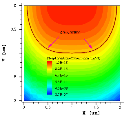
Figure 10. Two-dimensional phosphorus distribution.

Various settings discussed in this section are selected in the project RefineControls by the Sentaurus Workbench parameters @DopRefType@ and @Value@.

For @DopRefType@ set to None, the mesh is generated without having a RefinementFunction specification included in the global Refinement section of the command file (the doping definition used in the command file is discussed in Section 2.8 Defining the Doping Profile):

Definitions { ...
  Refinement "global" {
    MaxElementSize = ( 0.2 0.2 0.2 )
    MinElementSize = ( 0.01 0.01 0.01 )
  }
}

...

Placements { ...
  Refinement "global" {
    Reference = "global"
    RefineWindow = material ["Silicon"]
  }
}

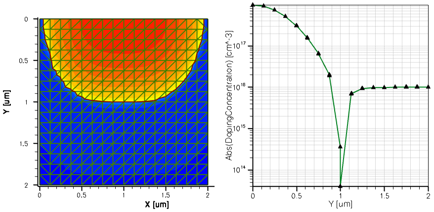
Figure 11. (Left) Two-dimensional uniform mesh and resulting doping profile distribution and (right) resulting doping profile on a uniform mesh, cut at x=1 coordinate across the p-n junction. (Click image for full-size view.)

As can be seen, the nonuniform part of the resulting doping profile is covered by only eight (8) mesh steps in the vertical direction, which is not sufficient to accurately resolve the profile spatial nonuniformity. In the end, such a coarse mesh will cause inaccurate results from the device electrical simulation and can lead to simulator failure.

For @DopRefType@ set to MaxTransDiff and @Value@ set to 1, the mesh is generated with an additional RefinementFunction statement in the Refinement description:

Definitions { ...
  Refinement "global" {
    MaxElementSize = ( 0.2 0.2 0.2 )
    MinElementSize = ( 0.01 0.01 0.01 )

    RefineFunction = MaxTransDiff(Variable="DopingConcentration", Value=@Value@)

  }
}

The MinElementSize parameter specifies the lower bound for the edge size of the mesh element in each spatial direction. These values are used for automatic mesh refinement on the doping. The RefineFunction statement activates the automatic mesh refinement based on the provided specification. In this particular case, the automatic refinement is based on the value difference of the resulting doping concentration. The keyword MaxTransDiff indicates that the hyperbolic arcsine function (asinh) should be used for the mesh refinement on doping.

The mesh refinement algorithm checks whether a function value difference between two neighboring mesh points is greater than a specified value (Value=1 in this case) and then refines the mesh accordingly.

Figure 12 shows the resulting mesh doping refinement, which was obtained with the above specification.

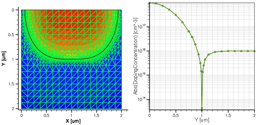
Figure 12. (Left) Two-dimensional mesh refinement on doping, showing the fine mesh resolution within the p-n junction area and (right) resulting doping profile cut at x=1 coordinate across the p-n junction, and the steep doping gradient is now much better resolved. (Click image for full-size view.)

Run the RefineControls project and view the generated mesh at the corresponding node with Sentaurus Visual.

As an alternative to the asinh (MaxTransDiff) function, the gradient of the function can be used as a refinement function. In this project, this is done for @DopRefType@ set to MaxGradient and @Value@ set to 1 (or 10). In this case, the mesh is generated with an additional RefinementFunction statement in the Refinement description:

Definitions { ...
  Refinement "global" {
    MaxElementSize = ( 0.2 0.2 0.2 )
    MinElementSize = ( 0.01 0.01 0.01 )

    RefineFunction = MaxGradient(Variable="DopingConcentration", Value=@Value@)

  }
}

If the gradient is greater than a specified value and the edge length is large enough, the element is refined. Figure 13 compares two meshes that were constructed with the MaxGradient doping refinement option using two different gradient values, namely, 1 and 10.

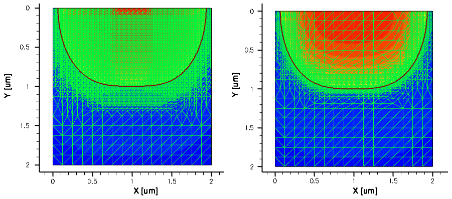
Figure 13. Refinement with (left) Value=1 and (right) Value=10. (Click image for full-size view.)

The refinement method used in Sentaurus Mesh is based on the binary tree, where each edge is split in two along a given direction until either a MinElementSize is fulfilled or required element aspect ratio criteria are fulfilled.

2.4 Interface Mesh Refinement

The Sentaurus Mesh command files featured in this section are all contained in the Sentaurus Workbench project Applications_Library/GettingStarted/snmesh/RefineInterface. To work with the project, copy it to a local directory within your Sentaurus Workbench working directory.

A frequently useful feature in Sentaurus Mesh is interface mesh refinement, which allows you to gradually resolve material interfaces in an isotropic manner.

The interface mesh refinement controls are embedded into a refinement region specification in the Definitions section:

Refinement "reference name" {
  MaxElementSize = (<xmax> <ymax> <zmax>)
  MinElementSize = (<xmin> <ymin> <zmin>)
  RefineFunction = MaxLengthInterface(Interface("<Material1>","<Material2>"),
                   Value = value, Factor = value [DoubleSide] [UseRegionNames])
}

where:

• Interface("<Material1>","<Material2>") indicates the materials whose interface must be refined.
• Value specifies the value of the initial mesh step at the interface.
• Factor controls the grading of the element sizes across the interface.
• DoubleSide (optional) initiates the mesh refinement on both sides of the interface. By default, the interface is refined inside <Material1> only.
• UseRegionNames (optional) interprets an interface as a regionwise specification.

Multiple RefineFunction definitions are allowed inside a single Refinement statement. Instead of the full MaxLengthInterface name, you can use MaxLenInt, for example:

Refinement "reference name" {
  MaxElementSize = (<xmax> <ymax> <zmax>)
  MinElementSize = (<xmin> <ymin> <zmin>)
  RefineFunction = MaxLenInt(Interface("Material1","Material2"),
                   Value = value, Factor = value)
}

In the RefineInterface project, the Sentaurus Mesh tool instance labeled IntRefA demonstrates the use of the interface refinement option in Sentaurus Mesh, where the interface refinement is applied to both sides of the silicon–SiO₂ and polysilicon–SiO₂ material interfaces:

Definitions {
  Refinement "global" {
    MaxElementSize = (1 1 1)
    MinElementSize = (0.01 0.01 0.01)
    RefineFunction = MaxLenInt(Interface("Silicon","SiO2"), 
             value=0.01, factor=2, DoubleSide)
    RefineFunction = MaxLenInt(Interface("PolySi","All"), 
             value=0.01, factor=2, DoubleSide)
  }
}

Figure 14. Interface mesh refinement. (Click image for full-size view.)

Click to view the command file IntRefA_msh.cmd.

The interface mesh refinement method works very well for axis-aligned or slightly nonaxis-aligned geometries. However, for strongly nonaxis-aligned device geometries, the interface mesh refinement can produce many mesh points while refining a nonplanar geometry, due to the specifics of the binary tree–based space decomposition, as shown in Figure 15.

Figure 15. Interface mesh refinement applied to nonaxis-aligned device geometry can produce a huge number of mesh points due to the specifications of the recursive binary-tree decomposition algorithm. (Click image for full-size view.)

In the RefineInterface project, the Sentaurus Mesh tool instance labeled IntRefB demonstrates the behavior of interface mesh refinement applied to a nonaxis-aligned device geometry.

Click to view the command file IntRefB_msh.cmd.

2.5 Offsetting

The possibility to generate boundary-conforming grids, using a combination of binary volume decomposition and offsetting algorithms, is implemented in Sentaurus Mesh.

The offsetting algorithm is activated by specifying the EnableOffset option in the IOControls section of the command file:

IOControls {
  EnableOffset
}

The controls for offsetting are specified in the Offsetting section of the command file:

Offsetting {
  noffset {
    hlocal = float
    factor = float
    maxlevel = integer
  }

  noffset material "<material_1>" "<material_2>" {
    factor = float
    hlocal = float
    window = [(float float float) (float float float)]
  }

  noffset material "<material_name>" {
    maxlevel = integer
  }
}

Both materialwise and regionwise specifications are supported.

The offsetting algorithm uses a combination of simple offsetting and level-set methods to generate mesh layers conformal with the device geometry.

Offsetting can be confined to a given window using a window specification. This often helps to maintain the best mesh quality for complex device structures. Note that a window controls only the starting position of layering and, therefore, layers can potentially grow outside of the window. Multiple window specifications within the same interface section are supported.

Figure 16 illustrates the most important offsetting parameters mentioned.

Figure 16. Main parameters related to offset layering at interfaces. At the material interface, the lateral mesh resolution is given by the axis-aligned mesh (AAM) refinement specifications. (Click image for full-size view.)

To illustrate how to use offsetting to generate a boundary-conforming anisotropic mesh layer, you will apply it to the same device structure, as shown in Figure 15. The maxlevel=6 specification has been applied to both the Silicon and Oxide materials, thereby creating six boundary-conforming mesh layers on both sides of the silicon–oxide interface. The layering starts with a layer thickness, specified by the hlocal value in the corresponding noffset material section. This setting applies to the first of two materials, which appear in each particular specification:

Offsetting {

  noffset material "Silicon" {
    maxlevel=6
  }

  noffset material "Oxide" {
    maxlevel=6
  }

  noffset material "Silicon" "Oxide" {
    hlocal=0.01
    factor=1.5
  }

  noffset material "Oxide" "Silicon" {
    hlocal=0.01
    factor=1.5
  }
}

The resulting boundary-conforming mesh is shown in Figure 17.

The Offsetting section in the command file is evaluated only if the IOControls section contains the EnableOffset or EnableSections option. Without one of these options, the Offsetting section is ignored and boundary-conforming layers are not produced.

Click to view the command file IntRefC_msh.cmd.

Figure 17. Boundary-conforming interface refinement applied to nonaxis-aligned device geometry by applying offsetting specifications at the silicon–oxide interface by Sentaurus Mesh. (Click image for full-size view.)

The Sentaurus Mesh tool instance labeled IntRefC, contained in the Sentaurus Workbench project Applications_Library/GettingStarted/snmesh/RefineInterface, demonstrates the behavior of interface mesh refinement applied to nonaxis-aligned device geometry. To work with the project, copy it to a local directory within your Sentaurus Workbench directory.

2.6 Multiboxes

Another method to define mesh refinement is a multibox, which is a special refinement box that is used to specify an isotropically graded refinement along one of the x-direction, y-direction, or z-direction. In general, using interface refinement (see Section 2.4 Interface Mesh Refinement) or offsetting (see Section 2.5 Offsetting) is easier than defining multibox refinement.

The syntax to define a multibox refinement in the Definitions section of the command file is:

Multibox "multibox reference name" {
  MaxElementSize = (<xmax> <ymax> <zmax>)
  MinElementSize = (<xmin> <ymin> <zmin>)
  Ratio = (ratio_x ratio_y ratio_z)
}

where:

• MaxElementSize and MinElementSize are the same step definitions as for the refinement region.
• Ratio controls the grading of the element size along each axis direction.

A simple example that demonstrates the use of a multibox to generate a gradual mesh is given in the project Refinements (see Section 2.2 Refinement Regions) at the Sentaurus Mesh tool instance labeled multibox1. It uses the same 2 μm x 2 μm silicon block device boundary as in the previous examples. Run the corresponding project node and view the generated mesh with Sentaurus Visual.

Definitions {
  Multibox "mb" {
    MaxElementSize = (1 1)
    MinElementSize = (0.1 0.1)
    Ratio = (1 2)
  }
}
Placements {
  Multibox "mb" {
    Reference = "mb"
    RefineWindow = rectangle[(0 0) (2 2)]
  }
}

Grading factors specified in the Ratio parameter control the gradual meshing in the corresponding direction. Having a grading factor higher than 1 (or lower than –1) means that the initial mesh step value, which is defined as MinElementSize, is used in the corresponding direction (in the above example, it is the y-direction). Each subsequent mesh step calculation is based on the formula step(i)=step(i-1)*ratio_factor.

If a ratio factor equals 1 exactly, grading is not produced, but the MaxElementSize step value is used instead. If a ratio factor equals 0 exactly, the corresponding specification is ignored. The mesh produced with the above specification is shown in Figure 18.

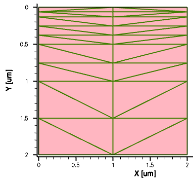
Figure 18. Mesh produced with multibox specification.

As you can see, the mesh grading is produced along the y-direction from the top to the bottom, following the multibox Ratio specification. The initial step value produced in this example differs from the specified one (it is smaller than 0.1 μm). This is again a result of the specifications of the binary-tree decomposition algorithm (see Section 2.2 Refinement Regions).

The next example demonstrates how you can use a negative grading ratio value to control the grading direction. The following changes were made to the multibox definition in the command file:

Definitions {
  Multibox "mb" {
    MaxElementSize = (1 1)
    MinElementSize = (0.1 0.1)
    Ratio = (2 -2)
  }
}

Having a y-axis ratio factor equal to –2 means that Sentaurus Mesh will change the grading direction from downwards to upwards. In addition, note how gradings in different directions can be combined. Arrows indicate the corresponding multibox grading directions (see Figure 19).

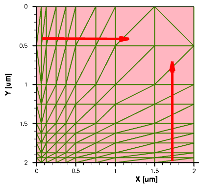
Figure 19. Multibox direction controls.

A demonstration of the use of multiboxes to generate gradings in different directions is given in the project Refinements (see Section 2.2 Refinement Regions) at the Sentaurus Mesh tool instance labeled multibox2. Run the corresponding project node and view the generated mesh with Sentaurus Visual.

2.7 Mesh Smoothing

By default, Sentaurus Mesh applies an automatic mesh-smoothing procedure when constructing a mesh to ensure that the mesh-element aspect ratio (the relative difference between adjacent mesh element edges) is maintained.

You can control mesh-smoothing by changing the parameters in the AxisAligned section of the Sentaurus Mesh command file, including:

AxisAligned {
  smoothing = true | false
  maxAspectRatio = float
  maxNeighborRatio = float
  minEdgeLength = float
  maxAngle = float
  geometricAccuracy = float
  decimate = true | false
  xCuts = floatlist
  yCuts = floatlist
  zCuts = floatlist
  fitInterfaces = true | false
}

where:

• smoothing switches on (true) or off (false) mesh smoothing. If smoothing=true (default), the binary tree uses the maxAspectRatio and maxNeighborRatio parameter values for the mesh step grading.
• maxAspectRatio specifies the maximum-allowed element aspect ratio in the binary tree (default is 1e6).
• maxNeighborRatio specifies the size ratio between adjacent elements (default is 2 in 2D, 4 in 3D).
• minEdgeLength sets the minimum-allowed element edge length produced on the boundary before delaunization (default is 1e-7 μm).
• maxAngle determines the maximum angle produced in the binary tree (default is 90° in two dimensions and 165° in three dimensions).
• fitInterfaces instructs Sentaurus Mesh to calculate the Cuts automatically by first refining along axis-aligned interfaces.

For the rest of the parameters of the AxisAligned section, refer to the Sentaurus™ Mesh User Guide.

The Applications_Library/GettingStarted/snmesh/Smoothing Sentaurus Workbench project demonstrates how mesh-smoothing controls work for the above examples. To work with this project, copy it to a local directory within your Sentaurus Workbench working directory.

The Sentaurus Mesh tool instances labeled NoSmooth and Smooth demonstrate the consequence of the smoothing deactivation for the previously shown device structure (see Figure 20).

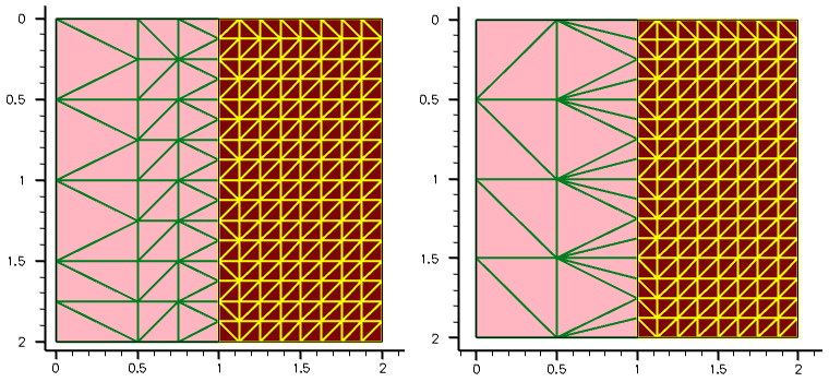
Figure 20. (Left) With smoothing=true and (right) with smoothing=false. (Click image for full-size view.)

Using smoothing=false, the mesh-step propagation from the material with the smaller step (oxide) towards the material with the higher step definition (silicon) is suppressed.

The next example illustrates the influence of the maxNeighborRatio parameter value on the mesh step smoothing for the previously shown example, with one order of magnitude step difference inside and outside the rectangular area, located in the middle of the device (see Figure 21).

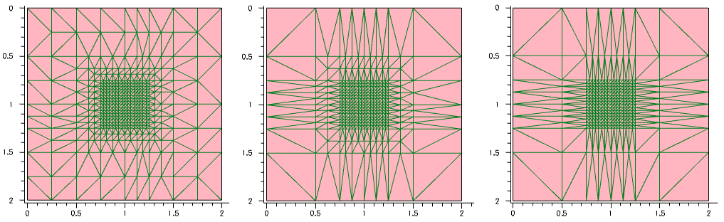
Figure 21. (Left) With maxNeighborRatio=2, (middle) maxNeighborRatio=4, and (right) maxNeighborRatio=8. (Click image for full-size view.)

The Sentaurus Mesh tool instance labeled NB_Ratio demonstrates the consequence of maxNeighborRatio control settings. Together with the smoothing control examples above, it is contained in the Applications_Library/GettingStarted/snmesh/Smoothing Sentaurus Workbench project.

2.8 Defining the Doping Profile

This section discusses aspects of 2D and 3D profile generation.

Examples of the Sentaurus Mesh features discussed in this section are all contained in the Sentaurus Workbench project Applications_Library/GettingStarted/snmesh/Profiles. To work with the project, copy it to a local directory within your Sentaurus Workbench working directory.

Sentaurus Mesh integrates the following profile generation–related capabilities:

• Generating 1D, 2D, and 3D profiles (doping, lifetime, mole fraction, stress, and so on) using constant or analytic profile descriptions, which substitute the necessity of having the numerically simulated profiles. This gives you quick access to a device simulation where a resulting profile is represented by the superposition of constant or analytic profiles.
• Having an interface between (2D or 3D) process and device simulators, allowing the transition of the doping profile from a process mesh to a mesh suitable for a device simulation.
• Constructing a 3D doping profile from 2D numerically simulated profiles using a profile sweep, slice, and rotation.
• Transferring a discrete doping profile, as a result of a kinetic Monte Carlo diffusion simulation, into a continuous doping profile to be used in a device electrical simulation.

2.8.1 Constant Profiles

A constant profile can be confined within a material, a region, or an arbitrary geometric element.

The first example demonstrates the concept of the constant profile definition on a simple 2D device structure, where the constant boron profile is confined within a rectangular window in the middle of the 2 μm x 2 μm silicon domain.

Figure 22 shows the profile variations performed with different lateral profile decays. Click to view the command files for the following Sentaurus Mesh tool instances in the Sentaurus Workbench project Profiles:

• Left image, zero decay length (DecayLength=0): Decay_Zero_msh.cmd
• Middle image, error function with 0.1 μm decay length (DecayLength=0.1): Decay_ErrFunc_msh.cmd
• Right image, Gaussian decay with 0.1 μm decay length (GaussDecayLength=0.1): Decay_Gauss_msh.cmd

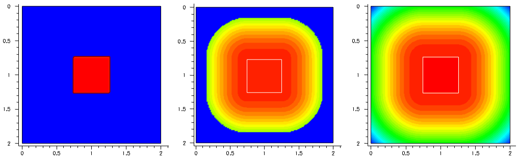
Figure 22. (Left) With DecayLength=0, (middle) DecayLength=0.1, and (right) GaussDecayLength=0.1. (Click image for full-size view.)

By default, the parameter DecayLength uses an error function, and GaussDecayLength uses a Gaussian function.

Figure 23 compares the profile cross-sections across the middle of the structure. Red-dashed lines indicate the locations of the constant profile primary domain.

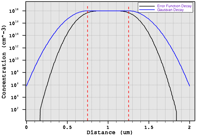
Figure 23. One-dimensional decay cross-section comparison. (Click image for full-size view.)

For more details about the constant profile definition, refer to the Sentaurus™ Mesh User Guide.

2.8.2 Analytic Profiles

The following example illustrates the concept of analytic profile definition. For 2D profiles, the reference region is defined using a baseline. The primary direction is the normal vector to the baseline, and the lateral direction is parallel to the baseline.

Figure 24 shows the schematics of the local coordinate system and the valid domain. The valid domain for both the primary and lateral functions is defined by sweeping the primary direction vector along the lateral direction. For a 3D analytic profile definition, instead of a baseline, a primary plane (or polygon) is used to define the reference region.

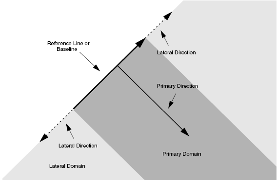
Figure 24. Concept of analytic profile definition.

The syntax for an analytic profile definition in the Definitions section is:

AnalyticalProfile "reference name" {
  Species  = "Dataset Name"
  Function = Gauss(parameters) | Erf(parameters) | subMesh1D(parameters) | 
             Eval(parameters) | General(parameters)
  LateralFunction = Gauss(parameters) | Erf(parameters) |
                    Eval(parameters)
}

where:

• Species indicates the species or variable name used for the analytic profile definition. Possible species names can be obtained from the datexcodes.txt file located in the $STROOT/tcad/$STRELEASE/lib directory.
• Function indicates the type of the component and its parameters used along the primary direction.
• LateralFunction defines the lateral component of the analytic profile.

For details about the analytic profile specification, refer to the Sentaurus™ Mesh User Guide.

Figure 25 demonstrates analytic profile definitions for a simple 2D device. The 2D profile baseline is specified in the middle of the device, as indicated by the white arrow. The Gaussian profile distribution has been chosen for the profile primary direction. In these examples, the profile primary domain and the lateral function distributions vary. By default, Sentaurus Mesh applies the profile on both sides of the baseline. Therefore, there is no need for a direction specification in the Placements section.

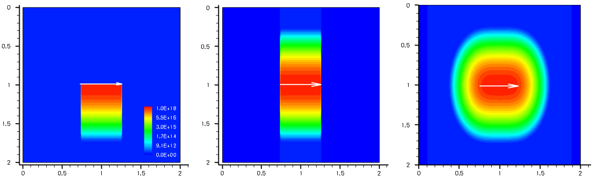
Figure 25. (Left) With Direction=positive, (middle) Direction=both, and (right) Direction=both and Erf(Factor=0.8). (Click image for full-size view.)

For Figure 25 (left), the analytic profile definition with a one-sided primary domain and disabled lateral profile distribution is:

Definitions { ...
  AnalyticalProfile "abc" {
    Species = "BoronActiveConcentration"
    Function = Gauss(PeakPos=0, PeakVal=1e+18, ValueAtDepth=1e15, Depth=0.5)
    LateralFunction = Erf(Factor=0)
  }
}

Placements { ...
  AnalyticalProfile "abc" {
    Reference = "abc"
    ReferenceElement {
      Element = Line [(0.75 1) (1.25 1)]
      Direction = positive
    }
  }
}

For Figure 25 (middle), the analytic profile definition with a double-sided primary domain and deactivated lateral profile distribution is:

Definitions { ...
  AnalyticalProfile "abc" {
    Species = "BoronActiveConcentration"
    Function = Gauss(PeakPos=0, PeakVal=1e+18, ValueAtDepth=1e15, Depth=0.5)
    LateralFunction = Erf(Factor=0)
  }
}

Placements { ...
  AnalyticalProfile "abc" {
    Reference = "abc"
    ReferenceElement {
      Element = Line [(0.75 1) (1.25 1)]
    }
  }
}

For Figure 25 (right), the analytic profile definition with a double-sided primary domain and activated lateral profile distribution is:

Definitions { ...
  AnalyticalProfile "abc" {
    Species = "BoronActiveConcentration"
    Function = Gauss(PeakPos=0, PeakVal=1e+18, ValueAtDepth=1e15, Depth=0.5)
    LateralFunction = Erf(Factor=0.8)
  }
}

Placements { ...
  AnalyticalProfile "abc" {
    Reference = "abc"
    ReferenceElement {
      Element = Line [(0.75 1) (1.25 1)]
    }
  }
}

Click to view the command files for the corresponding Sentaurus Mesh tool instances for these examples:

• Direction_A: Direction_A_msh.cmd
• Direction_B: Direction_B_msh.cmd
• Direction_C: Direction_C_msh.cmd

All of these command files are available in the Sentaurus Workbench project Applications_Library/GettingStarted/snmesh/Profiles.

The next example illustrates the analytic profile definition for a 3D device with the polygonal region used as the primary plane.

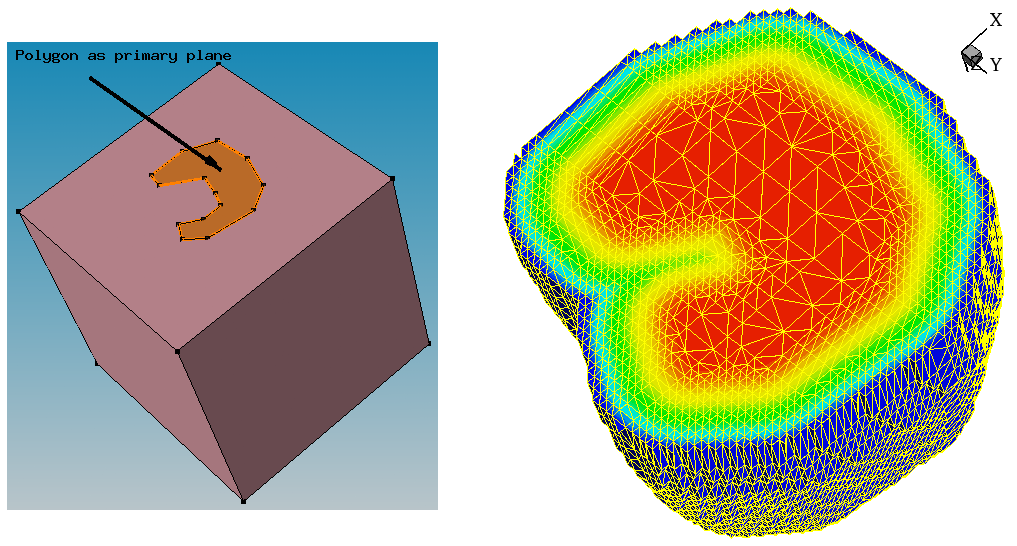
Figure 26. (Left) Polygonal region definition as a primary domain defined with Sentaurus Structure Editor and (right) resulting boron profile and 3D mesh as shown by Sentaurus Visual; the Value Blanking option is used to show the profile inside the device. (Click image for full-size view.)

Click to view the command file for the Sentaurus Mesh tool instance Polygon Polygon_msh.cmd.

Together with the above examples, this command file is contained in the Sentaurus Workbench project Applications_Library/GettingStarted/snmesh/Profiles.

2.8.3 Profile Overlap Controls

By default, the specified profiles are superimposed when they overlap. Switching on the Replace option allows you to change this behavior. In this case, the order in which profiles are placed is important. The next example demonstrates the use of the profile overlap controls. Three constant profiles are introduced that overlap (see Figure 27).

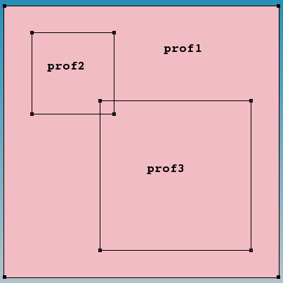
Figure 27. "prof1" is the background constant boron doping profile with 1e16 cm^-3 concentration; "prof2" is the constant boron doping profile with 1e18 cm^-3 concentration; and "prof3" is the constant arsenic doping profile with 1e18 cm^-3 concentration.

Figure 28 shows the resulting doping profile distributions (Nr = Ndonor – Nacceptor), illustrating the Sentaurus Mesh behavior when different overlap control scenarios are used:

• For Scenario A, the profile order, that is, how they appear in the Placements section of the command file, corresponds to the profile numbering, together with the default rule for profile overlay, which requires a profile sum at any spatial mesh vertex position. Therefore, for the area where high-doped boron and arsenic doping profiles overlap, the resulting doping profile concentration is equal to the background low-doped boron concentration (shown in light blue).
• For Scenario B, the same profile order is used as in Scenario A but the Replace option is specified for the prof2 profile. Therefore, the prof2 profile replaces the previously placed prof1 profile and then is overlapped with the prof3 profile, which results in zero net doping concentration within the overlay region (shown in green).
• Scenario C differs from Scenario B by adding the Replace option to the prof3 profile specification. In this case, the prof3 profile replaces both underlying boron profiles, as can be seen from the image.
• For Scenario D, the order, that is, how the profiles prof2 and prof3 appear in the command file, is changed compared to Scenario C, which results in the prof2 profile winning over other profiles.

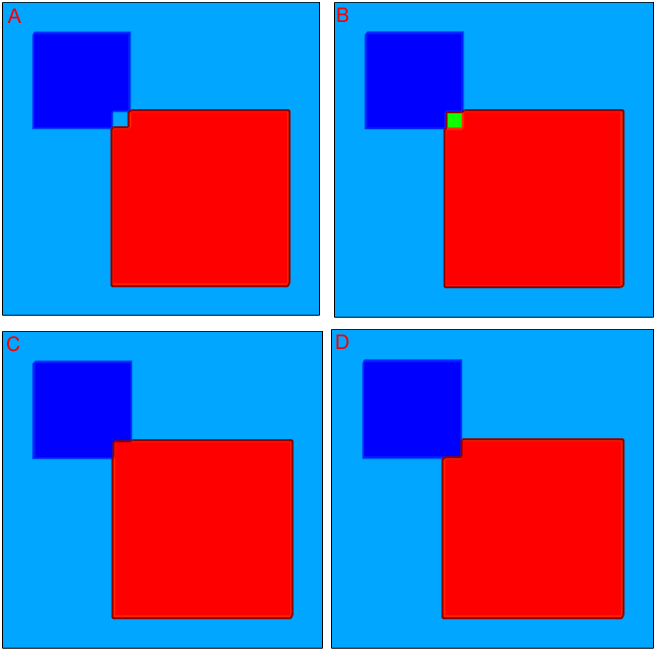
Figure 28. (Upper left) Scenario A, (upper right) Scenario B, (lower left) Scenario C, and (lower right) Scenario D. (Click image for full-size view.)

The Sentaurus Mesh command files featured in this section are all contained in the Sentaurus Workbench project Applications_Library/GettingStarted/snmesh/ProfileOverlap. To work with the project, start Sentaurus Workbench and copy the project ProfileOverlap to a local directory within the Sentaurus Workbench working directory.

Click to view the command files for the different scenarios for this example:

• Scenario A: OverlapA_msh.cmd
• Scenario B: OverlapB_msh.cmd
• Scenario C: OverlapC_msh.cmd
• Scenario D: OverlapD_msh.cmd

2.8.4 Submeshes

External simulation results from either a process or a device simulation can be used to refine the mesh to make it suitable for a subsequent device simulation.

The external profiles, which are the results of a 1D, 2D, or 3D process or device simulation, defined on a discrete mesh are called submeshes.

There are two distinctive submesh definitions in Sentaurus Mesh:

• External 1D profiles are used to construct 2D or 3D profiles using the analytic profile description (see Section 2.8.2 Analytic Profiles). Therefore, a 1D submesh is placed along the primary direction. For the lateral directions outside a primary domain, analytic functions are used.
• External profiles have the same spatial dimension as a target device. The datasets defined on the external mesh then are interpolated to the newly generated mesh.

The following example demonstrates how to incorporate an external 1D profile into a 2D device using the analytic profile description. The external 1D arsenic profile shown in Figure 29 (left) is incorporated into the 2D device structure using the subMesh1D option:

Definitions { ...
  AnalyticalProfile "AnalyticalProfileDefinition_1" {
    Function = subMesh1D(datafile = "1d_As.plx", scale = 1)
    LateralFunction = Gauss(Factor = 0.2)
  }
}

This example is contained in the Sentaurus Workbench project Applications_Library/GettingStarted/snmesh/SubMeshes.

Click to view the command file of the Sentaurus Mesh tool instance SubMesh1d SubMesh1d_msh.cmd.

The red arrow in Figure 29 (right) indicates the position of the 1D profile baseline. Outside the primary domain, the Gaussian profile distribution is used with a 0.2 factor with respect to the profile standard deviation along the primary direction.

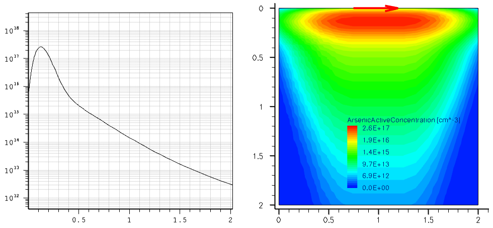
Figure 29. (Left) Referenced 1D arsenic profile and (right) resulting 2D doping profile with red arrow indicating the location of the profile baseline. (Click image for full-size view.)

The next example demonstrates how to incorporate a 2D external profile as a submesh to construct the mesh or doping profile suitable for device simulation. The Sentaurus Workbench project SubMeshes from the Applications_Library directory will be used here.

The goal of this example is to generate a mesh suitable for a device electrical simulation and to interpolate the doping and stress distributions from the original process grid onto the newly generated mesh. Due to the device symmetry, only half of the structure was simulated by Sentaurus Process (see the Sentaurus Process module). The structure remeshing was performed using the SubMesh option:

Definitions { ...
  SubMesh "SubMesh" {
    Geofile = "submesh_input2.tdr"
  }
}

Each individual dopant as well as stress components are interpolated from the original to the newly generated mesh. The original arsenic doping inside the poly gate is replaced by the constant doping using the Replace option:

  Constant "PlaceCD.Gate" {
    Reference = "Const.Gate"
    Replace
    EvaluateWindow {
      Element = material ["PolySi"]
      DecayLength = 0
    }
  }

The original grid and the resulting doping distribution after Sentaurus Process are shown in Figure 30 (left). The resulting mesh and the doping distribution, ready for Sentaurus Device, are shown in Figure 30 (right).

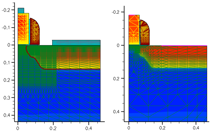
Figure 30. (Left) Original 2D mesh and doping profile from Sentaurus Process and (right) final mesh and doping profile distribution after Sentaurus Mesh. (Click image for full-size view.)

This example is contained in the Sentaurus Workbench project Applications_Library/GettingStarted/snmesh/SubMeshes.

Click to view the command file of the Sentaurus Mesh tool instance SubMesh2d SubMesh2d_msh.cmd.

To simulate the MOSFET device electrical behavior, the structure and mesh are mirrored at the x=0 axis location by Sentaurus Data Explorer, using the command:

tdx -mtt -x -ren drain=source test2d_half_subm_msh test2d_subm_msh

Alternatively, you can use the reflection capabilities of Sentaurus Mesh (see Section 4.2.4 Reflection).

This guarantees perfect mesh symmetry for the resulting device structure (see Figure 31).

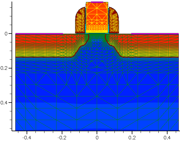
Figure 31. Mirrored device. (Click image for full-size view.)

An important feature of the SubMesh option is how the profile extrapolation is handled when the SubMesh domain and the target device geometries do not match (see Figure 32 (left)). In this case, Sentaurus Mesh extrudes all profiles outside the SubMesh domain, having them uniformly distributed, as shown in Figure 32 (right).

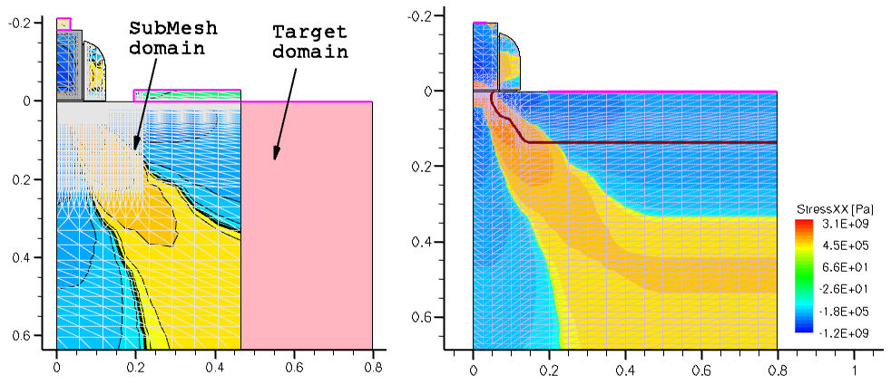
Figure 32. (Left) Mismatch of SubMesh and target device domains and (right) StressXX component of the stress tensor after remeshing. (Click image for full-size view.)

The next example demonstrates the use of the Ignoremat option of SubMesh.

The standard behavior of submesh interpolation is that the interpolation occurs only if the mesh vertex in a target device belongs to the same material as in a submesh device. If materials in a submesh device and a target device at the same vertex location are different, the profile interpolation for this vertex is suppressed. To overcome this limitation, you can specify Ignoremat in a submesh Placements section, which instructs Sentaurus Mesh to allow a profile interpolation, regardless of whether the materials match or do not match:

Placements {...
  SubMesh "SubMesh" {
    Reference = "SubMesh"
    Ignoremat
  }
}

Figure 33 demonstrates this behavior. The remeshing is performed for the target device, which differs from the submesh device by having a polysilicon region in the middle of the structure instead of silicon.

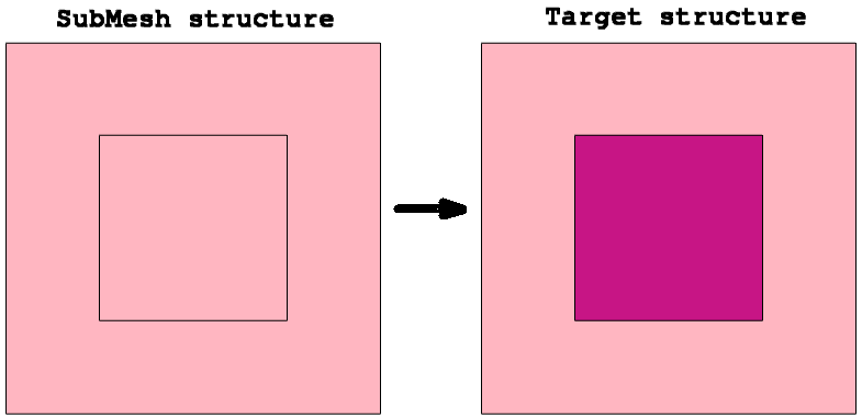
Figure 33. Test cases showing effect of Ignoremat. (Click image for full-size view.)

Figure 34 shows the results of interpolation. The submesh device is uniformly doped with boron (left image). By default, Sentaurus Mesh suppresses the doping interpolation inside the polysilicon material for the target device (middle image). Switching on the Ignoremat option activates the interpolation inside nonmatching materials and produces exactly the same profile as in the submesh (right image).

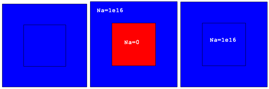
Figure 34. (Left) Submesh device with uniform 1e16 boron doping distribution, (middle) target device showing Sentaurus Mesh default interpolation behavior and boron concentration inside polysilicon is suppressed, and (right) demonstration of Ignoremat behavior and boron doping is also interpolated inside polysilicon material. (Click image for full-size view.)

Besides the submesh interpolation schemes previously described, you can specify the option MatchMaterialType:

Placements {...
  SubMesh "SubMesh" {
    Reference = "SubMesh"
    MatchMaterialType
  }
}

When MatchMaterialType is specified, the submesh attempts to match equivalent material types (for example, semiconductor-semiconductor, insulator-insulator, conductor-conductor) instead of trying to match material names when looking up values from which to interpolate.

The last example illustrates the Sentaurus Mesh capability to remesh the device, using the previously obtained device simulation result taken as a submesh.

It often happens that a device needs remeshing after device simulation, based on a solution of a certain carrier transport task. In this example, the remeshing is based on the profile of the carrier impact ionization rate, obtained on a coarse mesh (see Figure 35 (left)). The peak ionization rate appears to be in a region with the coarse mesh that needs to be remeshed. This solution is taken as a submesh, then the mesh refinement based on the impact ionization values within a given range is used as a refinement criterion together with the mesh refinement on doping:

Definitions {
  Refinement "Default Region" {
    MaxElementSize = (1 1 )
    MinElementSize = (0.05 0.05 )
    RefineFunction = MaxInterval(
      Variable = "ImpactIonization", 
      cmin=1e20, cmax=1e30, targetLength=0.05, 
      scaling=1, rolloff
    )
    RefineFunction = MaxTransDiff(Variable="DopingConcentration", Value=1)
  }
  ...
}

The option is activated with the MaxInterval keyword, where Variable defines the dataset field name, on which the mesh refinement is produced. cmin and cmax define the interval values to be considered by the refinement procedure. The algorithm analyzes each edge in a refinement tree cell and refines the edge if the data values at the endpoints overlap a given interval and the edge is longer than the maximum edge length, defined by the targetLength value, which sets the constant mesh resolution within the given range of field values. The coarser value between MinElementSize and targetLength is used in this case.

With rolloff switched on, the scaling parameter value determines how the mesh step transition towards the outside of the refinement domain is applied, according to the following formula:

targetLengthOutside = targetLength*(1 + log(Ca) - log(Cb))^2 * scaling

where Ca and Cb are the variable values at the endpoints of the edge.

The resulting mesh, shown in Figure 35 (right), demonstrates the finer mesh refinement within the area with large values of the impact ionization rate and large doping profile gradients.

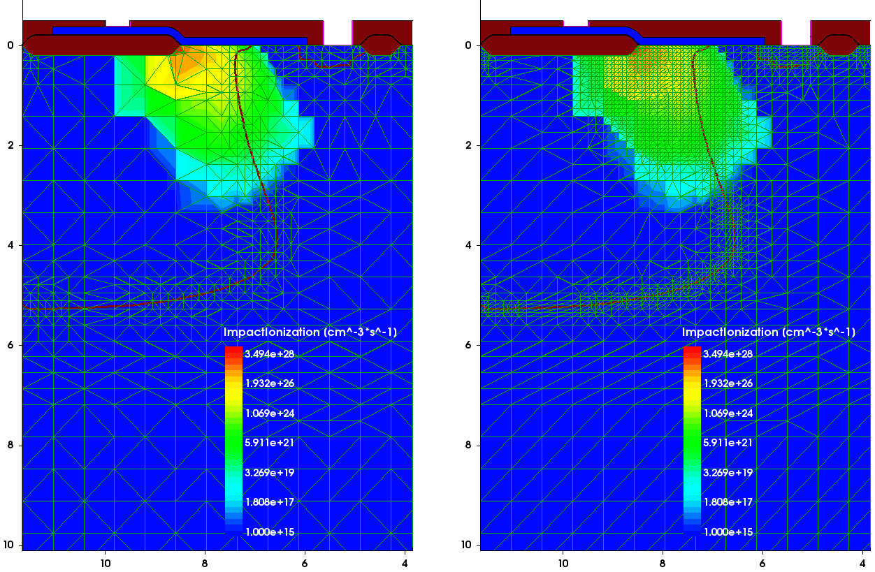
Figure 35. (Left) The previously calculated carrier impact ionization rate distribution on a coarse mesh is taken as a submesh for mesh adaptive refinement and (right) the mesh adapted to the impact ionization rate profile after remeshing. (Click image for full-size view.)

This example is contained in the Sentaurus Workbench project Applications_Library/GettingStarted/snmesh/SubMeshes.

Click to view the command file of the Sentaurus Mesh tool instance SubMesh2dII SubMesh2dII_msh.cmd.

2.8.5 Doping Naming Conventions

Transferring doping profiles from Sentaurus Process to Sentaurus Device using the Sentaurus Mesh SubMesh option is relatively straightforward. However, the doping profile compilation with constant or analytic profiles requires a certain naming convention to guarantee that profiles are handled properly by the device simulator.

Sentaurus Mesh uses active donor and acceptor dopants to calculate the resulting (net) doping profile (Nr):

Nr = Sum(Nd) - Sum(Na)

where:

• Sum() is the sum of all present dopants of either donor or acceptor type for each mesh vertex spatial location inside the device structure.
• Nd is an active donor dopant concentration.
• Na is an active acceptor dopant concentration.

For silicon material as well as for other semiconductors from group IV of the periodic table of elements, special names are reserved for donor and acceptor dopants, which are defined in the $STROOT/tcad/$STRELEASE/lib/datexcodes.txt file.

For donor dopants, the most important names are:

• AntimonyActiveConcentration
• ArsenicActiveConcentration
• PhosphorusActiveConcentration

For acceptor dopants, the most important names are:

• AluminumActiveConcentration
• BerylliumActiveConcentration
• BoronActiveConcentration
• IndiumActiveConcentration

While constructing doping profiles, Sentaurus Mesh calculates the resulting (net) doping profile applying the previous formula and saves individual dopants and the resulting doping profile in a TDR file. For each individual dopant, its profile is interpolated to a final mesh. However, for a resulting doping profile, the following rules apply:

1. If a dopant is defined that has one of the mentioned names, it is used for a resulting doping profile calculation.
2. If there are no profiles with the mentioned *ActiveConcentration names, Sentaurus Mesh checks whether there are corresponding profiles with total concentrations *Concentration, for example PhosphorusConcentration, and uses them to calculate a resulting doping profile.
3. If a profile called DopingConcentration is specified in the command file, it is summed with the resulting doping profile calculated with the previous formula.
4. If there are dopants with the names NDopantActiveConcentration or PDopantActiveConcentration defined, they are used as donor and acceptor dopants, respectively, in the resulting doping calculation.

The latter rule allows you to specify the doping distribution for III–V or II–VI semiconductor materials, such as GaAs and HgTe, and their compounds.

The following examples illustrate these naming conventions. The same structure and profile definitions as in the example in Section 2.8.3 Profile Overlap Controls are used here.

Four cases with different profile names were defined (see Figure 36):

• For Example 1, all profiles are defined as active. These values indicate the resulting doping concentration at each profile location. The background net doping concentration within the area indicated as prof1 is negative, since only BoronActiveConcentration doping (acceptor type) is specified there. For overlapping profiles, the doping superposition is applied according to the above formula.
• For Example 2, the BoronConcentration species name has been chosen for the prof1 profile instead of BoronActiveConcentration, as in Example 1. Since there are still active dopant specifications defined for the prof2 and prof3 profiles, the prof1 profile definition is ignored when the resulting doping profile calculation is performed (you can see that the doping profile value inside the prof1 domain is zero).
• For Example 3, the species name for the prof1 doping profile is DopingConcentration. Therefore, the resulting net doping is calculated according to Rule 3 as a superposition of the individual active dopants and the prof1 doping profile.
• For Example 4, the NDopantActiveConcentration and PDopantActiveConcentration names are used instead of BoronActiveConcentration and ArsenicActiveConcentration to define the doping profile. As can be seen, such definitions produce exactly the same resulting doping profile, as in Example 1.

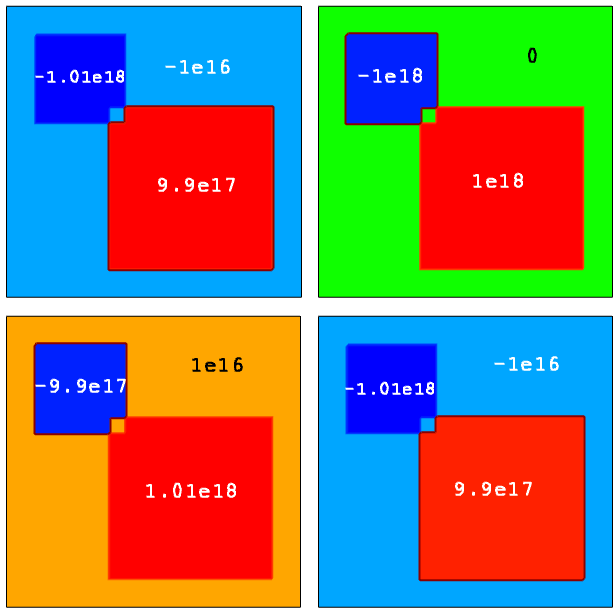
Figure 36. (Upper left) Example 1, (upper right) Example 2, (lower left) Example 3, and (lower right) Example 4. (Click image for full-size view.)

The Sentaurus Mesh command files featured in this section are in the Sentaurus Workbench project Applications_Library/GettingStarted/snmesh/DopingNameConventions. To work with the project, start Sentaurus Workbench and copy the project DopingNameConventions to a local directory within the Sentaurus Workbench working directory.

Click to view the command files for the different examples:

• Example 1: nameA_msh.cmd
• Example 2: nameB_msh.cmd
• Example 3: nameC_msh.cmd
• Example 4: nameD_msh.cmd

2.9 Advanced Options

In this section, some advanced options of Sentaurus Mesh are discussed including:

• Mesh delaunization
• General function evaluator
• Some aspects of 3D doping profile construction
• Discrete-to-continuous dopant profile transition

2.9.1 Mesh Delaunization

Mesh delaunization is a mandatory meshing step. It produces final grids suitable for the box discretization method, which is used in Sentaurus Process and Sentaurus Device. Delaunization is the most critical part in the case of 3D meshing, which requires some occasional compromises to produce a suitable mesh in terms of quality and size (node count). For 2D meshing, fully Delaunay grids are usually produced.

The delaunization step focuses on several targets. The major ones are:

• Each mesh element must meet the Delaunay triangulation criterion. This ensures that convergence is maintained on the simulator side.
• Slivers (elements with zero volume) must be eliminated.
• You must control the average node connectivity.
• During delaunization, the aspect ratio of neighbor elements is maintained.

Delaunay Triangulation Criterion Delaunay triangulation requires that the smallest circumscribed sphere around the element boundary faces and ridges must be free of points. This ensures that the following key features in the numeric 2D or 3D process or device simulators are guaranteed: There is mass conservation within each control volume. The material-dependent properties are encapsulated properly. The normal fluxes across the control surfaces can be evaluated easily.

The delaunization step controls are in the Delaunizer section of the Sentaurus Mesh command file:

Delaunizer {
  coplanarityAngle = float
  coplanarityDistance = float
  delaunayTolerance = float
  edgeProximity = float
  faceProximity = float
  maxAngle = float
  maxConnectivity = float
  maxNeighborRatio = float
  maxPoints = integer
  maxSolidAngle = float
  maxTetQuality = float
  minAngle = float
  minEdgeLength = float
  sliverAngle = float
  sliverDistance = float
  storeDelaunayWeight = true | false
  type = boxmethod | conforming | constrained
}

where:

• The parameter type specifies which type of Delaunay mesh must be produced:
  
  • boxmethod (default): Imposes the strictest conditions on the boundaries, requiring an almost ideal Delaunay mesh to be produced.
  • conforming: Equivalent to the standard Delaunay condition, where more relaxed conditions are used for the boundaries of the element.
  • constrained: Produces the least refinement of all these options. The meshes are often unsuitable for device simulation.
  
  In most cases, the default method produces the best quality meshes. In some situations, making a mesh slightly non-Delaunay helps to drastically reduce the node count without sacrificing simulator accuracy.
• The parameter delaunayTolerance uses a floating-point number (it must be between 0 and 1) to specify how close the ridges and boundary faces conform to the Delaunay criterion. A value of 0 implies a very strict Delaunay criterion. A value of 1 is equivalent to the construction of a constrained Delaunay triangulation (CDT). The delaunayTolerance can be defined materialwise or regionwise. For example, the following specification activates the CDT in oxide material only, while everywhere else the boxmethod Delaunay triangulation is used:
  

  Delaunizer {...
    delaunayTolerance=0
    interior material "Oxide" {delaunayTolerance=1}
  }
  

• The parameter maxPoints sets a limit on the maximum number of vertices that the delaunizer generates (default is 100000). Be careful because, when meshing a large 3D device, this value can be exceeded easily. In this case, the delaunizer will stop a triangulation and the final mesh might be non-Delaunay.
• The parameters maxAngle and minAngle specify the maximum and minimum angles allowed, respectively, in mesh elements (2D only).
• The parameter minEdgeLength sets the threshold for the minimum-allowed element edge length (default is 1e-9 μm).
• The parameter maxNeighborRatio specifies the maximum-allowed ratio between the circumscribed spheres of neighbor elements. It can be used in combination with the maxNeighborRatio option of the AxisAligned section for better mesh grading (default is 2 in 2D, 4 in 3D).

For the rest of the parameters of the Delaunizer section, refer to the Sentaurus™ Mesh User Guide.

Figure 37 shows the results of varying the value of minAngle for the previously shown example.

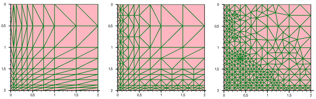
Figure 37. Mesh with minAngle equal to (left) 5°, (middle) 15°, and (right) 30°. (Click image for full-size view.)

2.9.1.1 Mesh Quality After Delaunization

For most 2D cases, a generated mesh will be 100% Delaunay, which is not the case for 3D device meshing. Different 3D mesh quality measures basically indicate whether a produced mesh is suitable for process or device simulation. You must perform a few simple checks to ensure that the following criteria are fulfilled:

• The produced node number does not exceed the given limit – by default 100000 mesh vertices. If this is the case, increase the maximal node number using maxPoints.
• The produced node number is still within a reasonable limit. It does not make sense to simulate a device with a million mesh vertices if there is not enough RAM available. For example, solving the carrier drift-diffusion transport task on a mesh with 100000 vertices requires approximately 4 GB of RAM. The same task on a mesh with 200000 vertices already requires approximately 16 GB of RAM.
• The maximal aspect ratio of the mesh element (the ratio of element edge sizes in different directions), in three dimensions, usually should be within the range 10–20. If the element aspect ratio is high, simulators sometimes experience convergence difficulties.
• The number of obtuse angles or flat elements in the mesh is zero or close to zero. Sentaurus Mesh produces a report about the mesh quality, showing the element maximal angle statistics in the form of the following text chart, which indicates the percentage of large-angle or small-angle elements:

================================== quality ========================================
 0  10  20  30  40  50  60  70  80  90  100  110  120  130  140  150  160  170  180
%  2   6   6   9   11  12  10  6   6   29    1    1    1    .    .    .    .    .
                                     |
                                     |
                                     |
                                     |
                                     |
                                     |
                                     |
                   |  |              |
               ||| |  | |||          |
               ||| |  | |||    |   | |
 -||||||||||||||||||||||||||||||||||||-----------------------------------
 0...1...2...3...4...5...6...7...8...9...1...1...1...1...1...1...1...1...1
     0   0   0   0   0   0   0   0   0   0   1   2   3   4   5   6   7   8
                                         0   0   0   0   0   0   0   0   0
---------------------------------------------------------------------------------

In addition, to verify the mesh quality after delaunization, you are advised to check the DeltaVolume report in the Sentaurus Device log file, which indicates how big is the difference between the real physical volume and the volume estimated by the box discretization method for each device region:

Region      Volume [um3]        BoxMethodVolume [um3]   DeltaVolume
--------------------------------------------------------------------
Poly        4.990000000000e-03  4.990000000000e-03      0.000000 %
OxideP      9.500000000000e-06  9.500000000000e-06      0.000000 %
Oxide       1.000000000000e-06  1.000000000000e-06      0.000000 %
OxideC      9.500000000000e-06  9.500000000000e-06      0.000000 %
Channel     4.990000000000e-03  4.990000000000e-03      0.000000 %
Total       1.000000000000e-02  1.000000000000e-02      0.000000 %

If the difference is greater than 2–5% for semiconductor regions, this can indicate that the mesh is not exactly Delaunay, which can cause a simulator convergence problem or inaccurate results. For insulator regions, the nonzero DeltaVolume values are less important.

2.9.2 General Function Evaluator

Apart from the predefined Gaussian and error functions, you can define an arbitrary general analytic function that can be used to define primary and lateral profile distributions for analytic profile definitions. The general function evaluator (GFE) uses the following syntax:

AnalyticalProfile "reference name" {
  Function = General(init="variable assignments", 
                     function="evaluated expression", 
                     value=<default_return_value>)
  LateralFunction = General(init = "variable assignments", 
                            function = "evaluated expression")
}

where:

• init is a semicolon-separated list of assignments for variables that are used in the Function expression.
• function is an expression that is evaluated for every query.
• value is the default return value if the evaluation fails.

The first example demonstrates the application of the GFE to construct a linearly graded doping profile. For the structure in Figure 38, the linearly graded phosphorus doping profile is defined inside the SiGe region, which is sandwiched between two uniformly doped silicon regions.

This example is contained in the Sentaurus Workbench project Applications_Library/GettingStarted/snmesh/EvaluateFunction.

Click to view the command file of the Sentaurus Mesh tool instance called linear linear_msh.cmd.

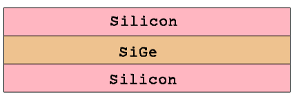
Figure 38. Test structure showing linear doping.

The following syntax specifies a linearly graded profile inside the SiGe region:

Definitions {
  AnalyticalProfile "linear" {
    Species = "PhosphorusActiveConcentration"
    Function = General( init = "fmax=10^18;fmin=10^16"  
        function = "10.*(fmin-fmax)*y+2.*fmax-fmin" value = 0)
  }
  ...
}

The function expression ensures that the profile values at the outer boundaries of the SiGe layer meet the specified boundary conditions: 1e18 cm^-3 at y = 0.1 μm and 1e16 cm^-3 at y = 0.2 μm.

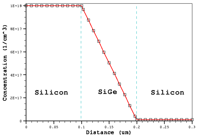
Figure 39. Linear doping and profile distribution. (Click image for full-size view.)

Click to view the command file layers1_dvs.cmd. Sentaurus Structure Editor uses this command file to produce such boundary and meshing commands.

The next example illustrates the use of the GFE to produce an automatic mesh refinement on an arbitrary function. In this example, the dummy profile is specified using the GFE:

  AnalyticProfile "dummy" {
    Species = "P2"
    Function = General(init="c0=10^5;lx=0.1;ly=0.1;lz=0.1",
               function="c0/exp((x/lx)^2)/exp((y/ly)^2)/exp((z/lz)^2)")
  }

The example uses the species called "P2", which is declared in the $STROOT/tcad/$STRELEASE/lib/datexcodes.txt file. The mesh refinement is based on the "P2" dummy profile distribution. The dummy 3D profile distribution and the final 3D mesh are shown in Figure 40.

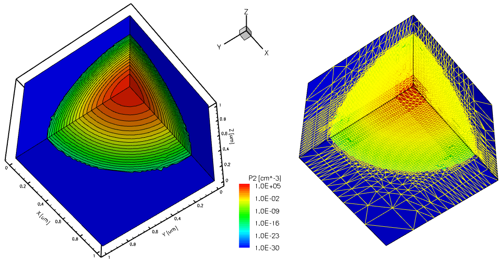
Figure 40. (Left) Dummy "P2" species profile generated by the GFE and (right) mesh adapted to the dummy profile distribution. (Click image for full-size view.)

This example is contained in the Sentaurus Workbench project Applications_Library/GettingStarted/snmesh/EvaluateFunction.

Click to view the command file for the Sentaurus Mesh tool instance GFEmesh GFEmesh_msh.cmd.

2.9.3 Three-Dimensional Doping Profile Construction

Sentaurus Mesh allows different 2D profile transformations such as rotation, extrusion, and sweeping. It is also possible to sweep a 2D geometry and a 2D profile along the same path simultaneously and to apply a similar sweep to the mesh refinement window for a more accurate mesh spatial discretization of a device.

The following example demonstrates the different techniques of 1D or 2D profile incorporation into a 3D device structure by applying several profile transformations, including 1D to 2D profile transfer, 2D profile rotation, extrusion, and sweeping.

The Sentaurus Mesh command files featured in this section are in the Sentaurus Workbench project Applications_Library/GettingStarted/snmesh/ProfileConstruction3D. To work with the project, start Sentaurus Workbench and copy the project ProfileConstruction3D to a local directory within the Sentaurus Workbench working directory.

As the first step, the 2D profile is created from the SubMesh1d profile using the analytic profile specification:

Definitions {
  AnalyticalProfile "AnalyticalProfileDefinition_1" {
    Function = subMesh1D(datafile = "1d_As.plx", scale = 1)
    LateralFunction = Gauss(Factor = 0.0)
  }
  ...
}

Placements {
  AnalyticalProfile "AnalyticalProfilePlacement_1" {
    Reference = "AnalyticalProfileDefinition_1"
    ReferenceElement {Element = Line [(-0.5 0) (1.5 0)]}
  }
  ...
}

The same 1D doping profile as described in Section 2.8.4 Submeshes is used here.

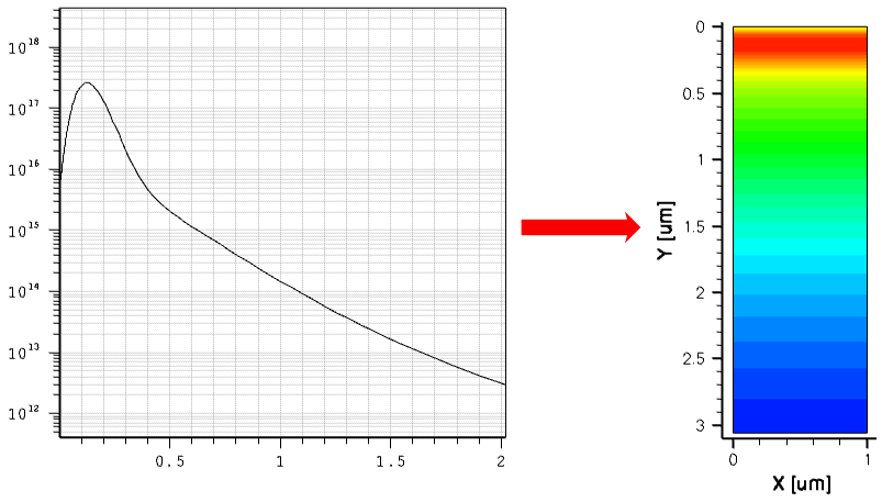
Figure 41. (Left) One-dimensional doping profile and (right) 2D profile. (Click image for full-size view.)

In the second step, the 2D profile is incorporated into the 3D domain using a combination of different submesh placements, involving a profile shift as well as rotation, sweeping, and replacement techniques (see Figure 42).

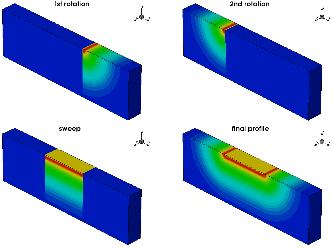
Figure 42. Three-dimensional profile construction technique. (Click image for full-size view.)

Click to view the command file rotsweep3D_msh.cmd. This command file produces the final 3D doping profile, shown in the lower-right image of Figure 42.

With the third step, the above 3D profile is cut using the Slice operation in the Tools section of the command file (see Section 4. Tools Section):

Tools {
  Slice {
    normal = (1 0 0)
    location = (0. 0. 0.)
  }
}

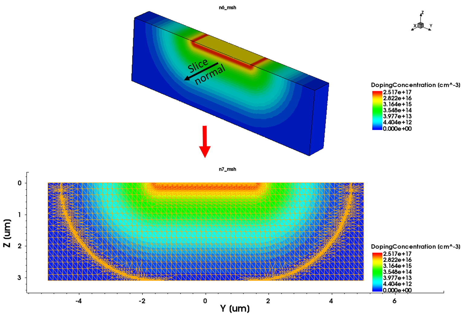
Figure 43. The result of a 2D cut using the Slice operation. (Click image for full-size view.)

Click to view the command file slice3Dto2D_msh.cmd. This command file produces the 2D doping profile shown in Figure 43 (right).

In the last step, the 2D profile is incorporated into the 3D device structure applying the profile rotation around the z-axis. The corresponding 3D device boundary is generated using Sentaurus Structure Editor.

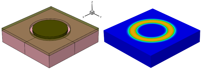
Figure 44. (Left) The 3D structure used for profile rotation and (right) the resulting 3D profile after rotation. (Click image for full-size view.)

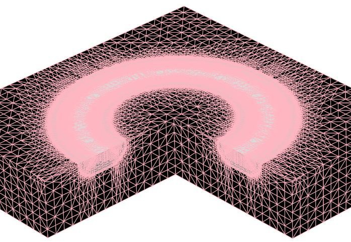
Figure 45. Resulting mesh after profile rotation. (Click image for full-size view.)

Click to view the command file make_torus_msh.cmd. This command file produces the 3D doping profile in Figure 45.

2.9.4 Discrete-to-Continuous Dopant Profile Transition

Sentaurus Mesh can create continuous doping profiles from discrete dopant distributions obtained using Sentaurus Process Kinetic Monte Carlo (Sentaurus Process KMC), which then can be used in device simulations.

Such a procedure is called deatomization, which is accomplished by associating a doping function with each discrete dopant. The union of all such doping functions defines the final doping profile.

The next example demonstrates the doping deatomization procedure. A 3D MOS transistor structure and atomized KMC species are shown in Figure 46. Note the Manhattan-type geometry of the originally rounded shapes, which is the result of using a tensor grid in the Sentaurus Process KMC simulation.

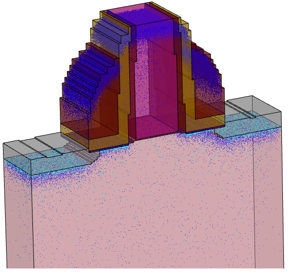
Figure 46. Result of 3D KMC simulation showing locations of the KMC species. Blue points indicate the location of single atom defects, mostly dopants. Cyan points indicate the location of impurity clusters. (Click image for full-size view.)

The discrete KMC results are loaded into Sentaurus Mesh where they are deatomized using a normalized charge density approach. The charge density functions for all dopants are then summed to form the final doping distribution to be used in a subsequent device simulation.

To deatomize the KMC dopants, the Particle section must be declared inside the Definitions section of the Sentaurus Mesh command file for each individual dopant. The following syntax illustrates the parameters of the Particle section to deatomize boron particles:

  Particle "BoronParticles" {
    ParticleFile = "kmc_final.tdr"
    Species = "BoronActiveConcentration"
    ScreeningFactor = 3.5e6
    AutoScreeningFactor
    Normalization
  }

where:

• ParticleFile indicates the location of the source for the boron particles profile, which is deatomized into BoronActiveConcentration.
• ScreeningFactor is the inverse of the screening length used for a profile deatomization.
• AutoScreeningFactor switches on an automatic screening factor calculation for each discrete dopant based on the local density of dopants.
• Normalization switches on the doping normalization for discrete dopants, whose doping function extends beyond the boundary.

Refer to the Sentaurus™ Mesh User Guide for details.

Figure 47 shows the results of the boron and arsenic profile deatomizations.

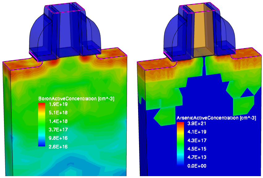
Figure 47. (Left) Deatomized boron profile after Sentaurus Mesh and (right) deatomized arsenic profile after Sentaurus Mesh. (Click image for full-size view.)

The complete project can be investigated from within Sentaurus Workbench in the directory Applications_Library/GettingStarted/snmesh/Deatomize.

Click to view the command file KMC_msh.cmd.

Right-click to save the TDR submesh file kmc_final.tdr from Sentaurus Process KMC (17 MB) used in this example.