 main menu
| module menu
| << previous section
| next section >>
main menu
| module menu
| << previous section
| next section >>
Sentaurus Visual
7. Special Focus: Fitting Dispersive Media for EMW
7.1 Overview
7.2 Basics of Fitting Dispersive Media
7.3 The emw::fit Library
7.4 Example: Fitting CRI Table for Different Materials
Objectives
- To understand the methodology of fitting materials with dispersive models in Sentaurus Device Electromagnetic Wave Solver (EMW).
- To learn how to use the emw::fit library of Sentaurus Visual.
7.1 Overview
The dispersive nature of light propagating through an absorbing material is typically characterized by a frequency-dependent complex refractive index (CRI). This CRI is directly specified using a wavelength-dependent table of n (index of refraction, real part) and k (extinction coefficient, imaginary part) values located in the material parameter file. Although the direct application of this CRI table in EMW simulations is allowed, it is important to understand how EMW uses this information and when it is necessary to fit the CRI to a dispersive media model before running simulations.
At wavelengths where the material is highly absorptive (k > n), EMW actually computes a negative value for the real part of the permittivity (Re[ε] = n2 – k2). This leads to numeric instability in the underlying finite-difference time-domain (FDTD) method implemented in EMW. To avoid this instability, EMW automatically adds a large value of conductivity, which forces the material to act like a perfect electric conductor. However, this auto-correction by EMW results in a change in the material property and effectively masks the dispersive nature of the material defined by the CRI table.
When a broadband EMW simulation is run with CRI tables specified, EMW uses the single values of n&k for the central wavelength of the broadband pulse throughout the entire simulation. The result is that the dispersive nature of the material over the simulated spectral range is not properly accounted for.
To avoid these problems, it is recommended that before running the EMW simulation, users perform a fitting of the CRI values using the available dispersive media models. The methodology of this fitting procedure is discussed and summarized in the next section.
Dispersive fitting of materials discussed next is required only for broadband simulations. Otherwise, the SingleDipoleDrude model can be used with the ComputeFromComplexRefractiveIndex feature to model dispersive materials. Refer to the simple2d-postprocess project in Section 2.11 Postprocessing for more details.
7.2 Basics of Fitting Dispersive Media
A proper fitting of a material's CRI to a specific dispersive media model is a necessary pre-simulation step to ensure stability and to improve the overall accuracy of EMW-computed optical absorption over a specific range of wavelengths. The basic methodology behind the fitting procedure is illustrated in Figure 1.
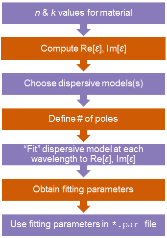
Figure 1. Fitting methodology for dispersive media.
The fitting procedure begins with reading in the n&k values from the CRI table in the material parameter file. Next, these values are used to compute the corresponding real and imaginary parts of the electric permittivity at each wavelength. Then, the values of permittivity are used along with a specific number of user-defined poles to fit the real and imaginary parts of the permittivity to a specific dispersive media model at each wavelength in the specified range of interest.
The end result of this procedure is a set of unique fitting parameters that are saved into a specific dispersive model section in a new material parameter file. During subsequent EMW simulations, these fitting parameters ensure that the dispersion of the modeled material over the simulated spectrum is correctly accounted for and that the underlying FDTD method will not encounter numeric instabilities due to negative permittivities as previously discussed.
7.3 The emw::fit Library
The emw::fit library of Sentaurus Visual is a Tcl-based module that is loaded and used within a Sentaurus Visual script. This library provides users with a way to specify all the parameters and settings necessary to fit a material's CRI table to a specific dispersive media model.
The library can be used directly from the Tcl Command panel, allowing users to:
- Modify all fitting parameters.
- Run material fittings.
- Plot all results.
During runtime, the emw::fit library reads in all the user-supplied parameters and performs a best fit of the material's CRI table to the specified dispersive model. When the fit is completed, the results can be automatically plotted (or updated) in the plot area of Sentaurus Visual.
In addition, the emw::fit library stores the current state of all parameters, which can later be dynamically modified from the user interface of Sentaurus Visual to accommodate "on-the-fly" changes that might be needed to improve the curve fitting to the available CRI data.
The next section presents an example that demonstrates how to use this library.
7.4 Example: Fitting CRI Table for Different Materials
This example demonstrates step-by-step how to set up and use the emw::fit library within a Sentaurus Workbench project to fit the CRI table of different materials to a specific dispersive media model over a particular range of wavelengths.
The example is divided into different tasks discussed in the following sections:
- Writing a Tcl script for the emw::fit library
- Running the fitting and visualizing the results
- Modifying the fitting parameters using the Tcl Command panel
The example is built around one Sentaurus Visual tool instance and a list of Sentaurus Workbench parameters associated with each of the fitting parameters. Figure 2 shows the workflow for the Sentaurus Workbench project for some materials.
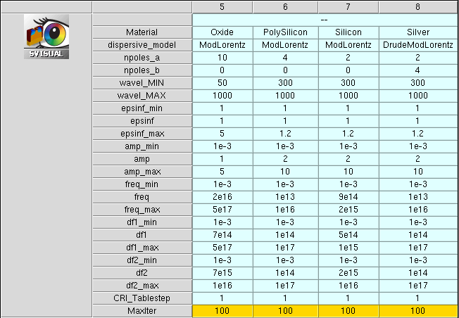
Figure 2. Workflow of Sentaurus Workbench project. (Click image for full-size view.)
7.4.1 Writing a Tcl Script for the emw::fit Library
You begin the script by loading the emw::fit library:
load_library emw_fit
Next, you define the following namespace:
namespace import emw::fit::*
This namespace definition allows you to type the names of procedures directly (for example, Globals) instead of typing the full procedure name (for example, emw::fit::Globals) each time. This will be important later when you want to change the fitting parameters using the Tcl Command panel.
Next, you define the following procedures:
- emw::fit::Globals
- emw::fit::ComplexRefractiveIndex
- emw::fit::Fitting
- emw::fit::DispersiveMedia
- emw::fit::Plot
Each procedure has the form emw::fit::<Procedure> –<keyword> <value>.
For example, the emw::fit::Globals and emw::fit::ComplexRefractiveIndex procedures are defined as:
emw::fit::Globals \
-CRITableFile  "par/@Material@.par" \
-ParameterFile "n@node@_fit.par" \
-ResultFile    "n@node@_fit.plt" \
-LogFile       "n@node@_fit.log"

emw::fit::ComplexRefractiveIndex \
-Material @Material@
The emw::fit:Globals procedure is mandatory and contains all of the global parameter settings for the input and output files. The input parameter file (.par) containing the CRI data and the output log file (.log) are specified by the keywords –CRITableFile and –LogFile, respectively. The output files into which the fitting parameters (.par) and the fitting results (.plt) are saved are specified by the keywords –ParameterFile and –ResultFile, respectively.
The emw::fit::ComplexRefractiveIndex procedure is mandatory. It contains the name of the material to which the selected dispersive media model is fitted and controls the wavelength dependencies of the CRI. The name of the material to be fitted is specified by the –Material keyword. The wavelength dependency can be controlled by the –WavelengthDep keyword. By default, the wavelength dependency is set to {Real Imag}.
The emw::fit::Fitting procedure is mandatory and specifies those parameters that directly control the performance or convergence behavior of the fitting algorithm. The configuration used in the example is:
emw::fit::Fitting \
-WavelengthRange      {@wavel_MIN@ @wavel_MAX@} \
-CRITableStep         @CRI_Tablestep@ \
-MaxIterations        @MaxIter@ \
-SimplexMaxFunEvals   @MaxFunEvals@ \
-SimplexMaxIterations 100000 \
-SimplexTolFun        1e-15 \
-WeightImagEps        2.0
The spectral range (–WavelengthRange) of the fitting is defined from 300 to 1000 nm. Each data entry (each set of wavelength-dependent n&k values) listed in the CRI table (–CRITableStep 1) will be used to fit the material using the specified dispersive model.
The maximum number of iterations (–MaxIterations) taken during the fitting procedure is limited to 100. The maximum number of objective function evaluations (–SimplexMaxFunEvals) and the maximum number of iterations (–SimplexMaxIterations) are each limited to 100000. This value is a reasonable starting point for most fittings. If a larger number of complex poles is specified or needed to obtain a better overall fit, you need to increase these values.
The convergence tolerance (–SimplexTolFun) is set to 1e-15.
Finally, the weighting factor for fitting the imaginary part of the permittivity (–WeightImagEps) is set to 2. Setting this factor to a value greater than 1 improves the quality of the fit for regions where the magnitude of the imaginary part of the permittivity is smaller compared to the real part.
The emw::fit::DispersiveMedia procedure is mandatory and defines the dispersive model and its fitting parameters. The setup used for the example is:
switch -exact -- [string tolower @dispersive_model@] {
  lorentz {
    emw::fit::DispersiveMedia \
    -Model                 Lorentz \
    -NumberLorentzPoles    @npoles_a@ \
    -EpsilonInf            { @epsinf@ @epsinf_min@ @epsinf_max@} \
    -LorentzAmp            { @amp@    @amp_min@    @amp_max@   } \
    -LorentzFreq           { @freq@   @freq_min@   @freq_max@  } \
    -LorentzDampFac        { @df1@    @df1_min@    @df1_max@   }
  }
  modlorentz {
    ...
  }
  ...
}
Here, you place a Tcl switch command around two different emw::fit::DispersiveMedia procedures. This setup allows you to choose either the Lorentz dispersive model, or the modified Lorentz dispersive model, or the Drude-modified Lorentz dispersive model by setting the @dispersive_model@ parameter of Sentaurus Workbench directly in the project workflow.
All of the fitting parameters for each dispersive model are uniquely specified in the form:
–<keyword> {<initial–value> <minimum–value> <maximum–value>}
In this example, you have parameterized all fitting parameters to accommodate multiple experiments in the Sentaurus Workbench projects.
ALL parameter values must be positive real and greater than zero. Otherwise, the emw::fit library will generate an error message, and the fitting procedure will fail to run.
For detailed descriptions of the dispersive media models and their fitting parameters, refer to the Sentaurus™ Device Electromagnetic Wave Solver User Guide, "Modeling of Dispersive Media".
The emw::fit::Plot procedure is optional and is used to specify when and how often a new fitting result plot is generated. If this procedure is omitted from the script, the library automatically generates a plot (.plt) file for the last iteration of the fitting procedure.
The following example starts plotting at 0 iterations and continues through the maximum number of iterations; a new plot is generated after every iteration. A final plot also will be generated after the last iteration is completed:
emw::fit::Plot \
  –StartTick  0 \
  –EndTick    @MaxIter@ \
  –TickStep   1 \
  –FinalPlot  yes
Finally, the following lines manage running the fit and plotting:
if {![info exists runVisualizerNodesTogether]} {
  emw::fit::Run
}
emw::fit::Graph
This instructs the library to run the fitting procedure when called in batch mode and then to plot automatically the results when you click the Run Selected Visualizer Nodes Together toolbar button.
Note that the Tcl variable runVisualizerNodesTogether is defined only if the script is called by clicking the Run Selected Visualizer Nodes Together toolbar button (compare with Section 6.5 Visualize Selected Nodes Together).
Click here to view the Sentaurus Visual Tcl script svisual_vis.tcl.
7.4.2 Running the Fitting Procedure and Visualizing the Results
Multiple different material-fitting experiments are provided in the Sentaurus Workbench project. For example, the first experiment fits aluminum using a 6-pole Drude-modified Lorentz model, and the seventh experiment demonstrates a fitting of silicon using a 2-pole modified Lorentz model. You will continue this module using the silicon example. The other examples are provided as additional examples that you can explore on your own.
Figure 3 shows the fitting results for silicon.
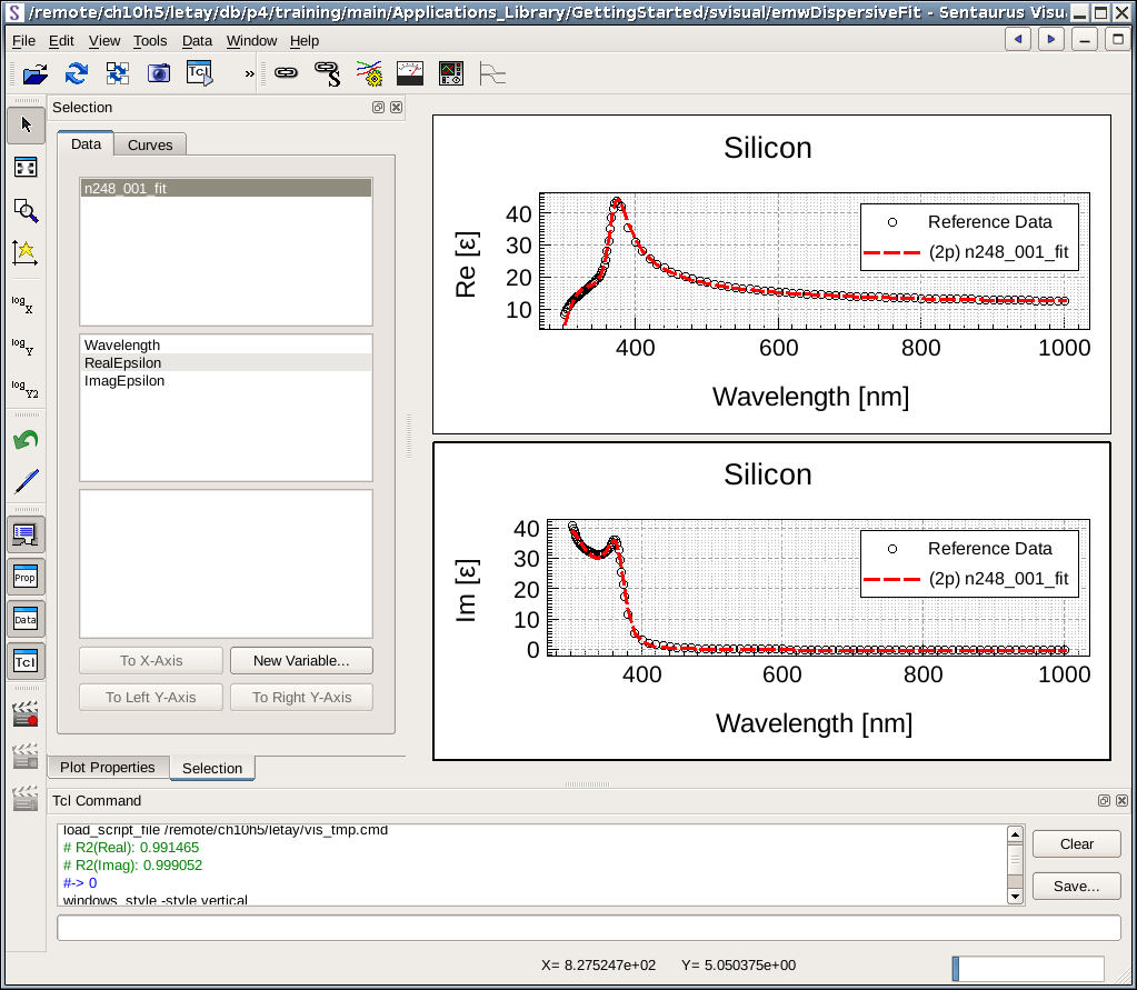
Figure 3. Silicon fit with 2-pole modified Lorentz model. (Click image for full-size view.)
The fitted curve is overlaid on top of the reference CRI data (denoted by open circles). The corresponding legend label for the fitted curve indicates that the results are for a 2-pole fit and that the fitting parameters are saved in the n46_001_fit.par file.
The quality of the fit for both the real and imaginary data, compared to the reference data, is shown in the Tcl Command panel of Sentaurus Visual.
You can always visualize already existing results, without rerunning the fit, by selecting the corresponding node in Sentaurus Workbench and clicking the Run Selected Visualizer Nodes Together toolbar button (compare with Section 6.5 Visualize Selected Nodes Together).
7.4.3 Modifying the Fitting Parameters Using Tcl Command Panel
All parameters specified in the Sentaurus Visual Tcl script can be modified directly in the Tcl Command panel. This allows you to make "on-the-fly" changes to adjust the quality of the fit.
When working interactively, at the beginning of the session,
execute the following line to allow you to use the commands directly, without
the emw::fit:: namespace:
namespace import emw::fit::*
For example, to rerun the fit of silicon using only 1 pole, simply modify the number of poles, and then rerun and replot the new results on the current plot. The sequence of procedures to accomplish this from the Tcl Command panel is:
DispersiveMedia -NumberModLorentzPoles 1  <press Enter key>
Run ; Graph  <press Enter key>
A new fitting is performed, and the results are updated as shown in Figure 4.
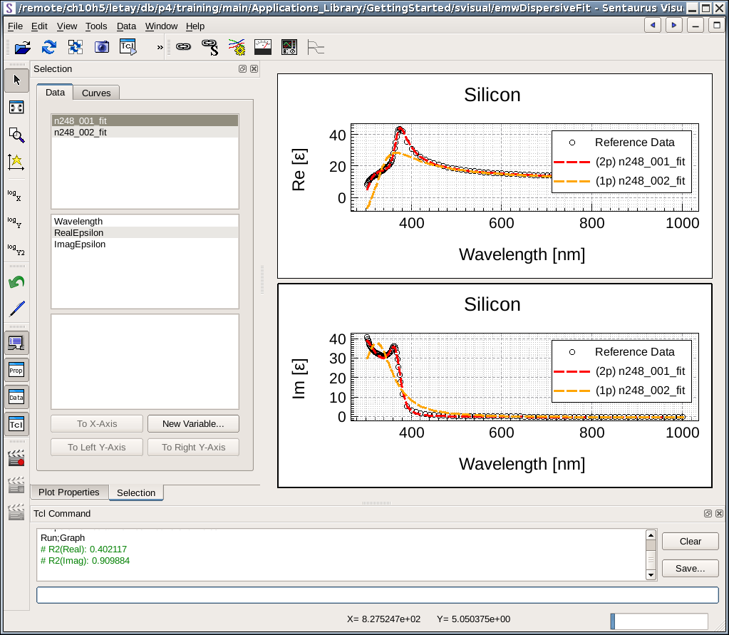
Figure 4. Updated silicon fit with 1-pole modified Lorentz model. (Click image for full-size view.)
Note that the label for the new fitted curve indicates that the results are for a 1-pole fit and that the new fitting parameters are saved in the n46_002_fit.par file.
To clear all the curve fittings and to replot only the last fitted curve, type the following commands in the Tcl Command panel:
Clear ; Graph <press Enter key>
This will update the plots as shown in Figure 5.
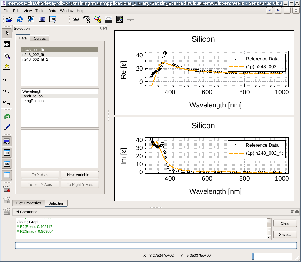
Figure 5. Reset plot to last fitted curve data. (Click image for full-size view.)
If, in an interactive session, a parameter must be removed again, assign the value remove to it. For example, to remove the parameter -numberMODLORENTZclowns from Dispersive, type the following in the Tcl Command panel:
Dispersive -numberMODLORENTZclowns remove
The complete project can be found within Sentaurus Workbench in the directory Applications_Library/GettingStarted/svisual/emwDispersiveFit.
main menu | module menu | << previous section | next section >>
Copyright © 2017 Synopsys, Inc. All rights reserved.