Sentaurus Structure Editor
3. Generating Doping Profiles

3.1 Defining Constant Doping Levels in Materials
3.2 Defining Constant Doping Levels in Regions
3.3 Defining Analytic Doping Profiles
3.4 Saving the Model
3.5 Assignment

Objectives

• To introduce the most important 2D doping definitions of Sentaurus Structure Editor using an SOI MOSFET.

3.1 Defining Constant Doping Levels in Materials

In this section, the SOI MOSFET built in Section 2. Generating 2D Boundaries will be used.

This section introduces the most basic approach to defining a constant background doping level within a material type.

To introduce a constant boron background doping of 1x10¹⁵ cm^-3 in the silicon material:

1. Choose Device > Constant Profile Placement.
   The Constant Profile Placement dialog box is displayed.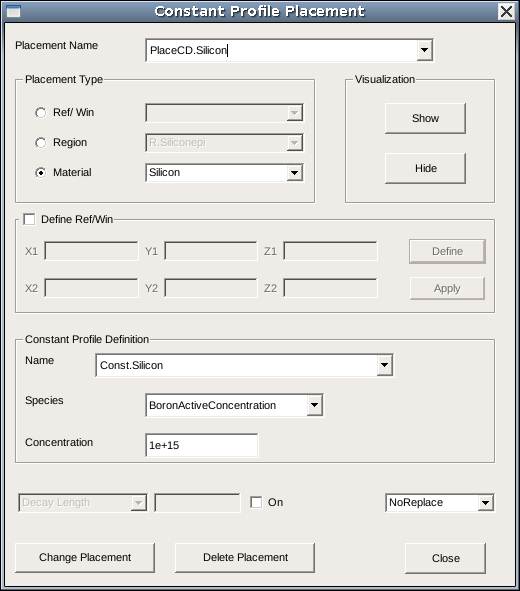

   

   Figure 1. Constant Profile Placement dialog box.

2. Type the name PlaceCD.Silicon in the Placement Name field.
3. Under Placement Type, select Material, and select Silicon as the region name.
4. Under Constant Profile Definition, type Const.Silicon in the Name field.
5. Select BoronActiveConcentration from the Species list.
6. Enter 1e15 in the Concentration field.
7. Click Add Placement to add the doping to the silicon substrate region.
8. Click Close.

The assignment of a constant doping profile to a specific material type involves, in general, two steps:

• The first step defines a constant profile, which in this case requires all the fields in the Constant Profile Definition group box to be completed.
• The second step associates the defined profile with a material type, which is performed by Sentaurus Structure Editor when you click the Add Placement button. However, before this step, both the placement type and the material type in the Placement Type group box must be selected.

The corresponding Scheme commands that reflect these two steps are:

(sdedr:define-constant-profile "Const.Silicon" "BoronActiveConcentration" 1e+15)
(sdedr:define-constant-profile-material "PlaceCD.Silicon" 
  "Const.Silicon" "Silicon") 

3.2 Defining Constant Doping Levels in Regions

The placement of a constant doping profile in a material adds the profile everywhere that the specified material resides. This can include more than one device region. Alternatively, you can assign a doping profile only to selected device regions.

To dope the silicon epilayer with a uniform boron concentration of 1x10¹⁷ cm^-3:

1. Choose Device > Constant Profile Placement.
   The Constant Profile Placement dialog box is displayed.
   

   

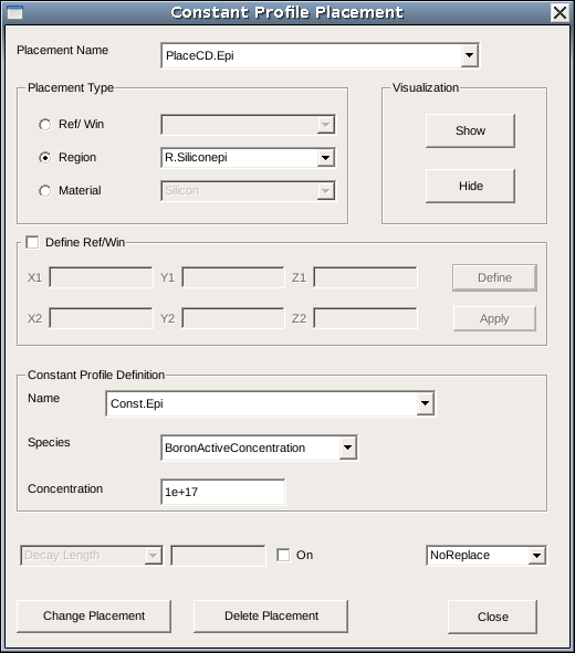
   Figure 2. Constant Profile Placement dialog box.

2. Type PlaceCD.Epi in the Placement Name field.
3. Under Placement Type, select Region, and select R.Siliconepi as the region name.
4. Under Constant Profile Definition, type Const.Epi in the Name field.
5. Select BoronActiveConcentration from the Species list.
6. Enter 1e17 in the Concentration field.
7. Click Add Placement.
8. Click Close.

The corresponding Scheme commands are:

(sdedr:define-constant-profile "Const.Epi" "BoronActiveConcentration" 1e17)
(sdedr:define-constant-profile-region "PlaceCD.Epi" "Const.Epi" "R.Siliconepi")

Constant doping profiles also can be applied to an evaluation window by selecting Ref/Win in the Placement Type group box. See Section 4.3 Defining Regional Refinements for instructions to define an evaluation window.

3.3 Defining Analytic Doping Profiles

In Sentaurus Structure Editor, you can define doping profiles characterized by analytic functions, such as Gaussian and error functions. In addition, you can define doping profiles of your own functions, which can be useful in some applications.

The placement of an analytic profile is performed usually in two steps. The first step defines the baseline and the second step defines the shape of the profile itself. The baseline determines the lateral extent of the profile and also can serve as the reference point for the depth of the peak position.

Two Gaussian doping profiles are to be added to the source/drain and their extension regions of the example structure. For the source/drain region, the target is a Gaussian phosphorus profile with a peak concentration of 5x10¹⁹ cm^-3, a junction depth of 0.12 μm, and a lateral straggle/diffusion factor of 0.8.

For the source/drain extensions, the goal is a Gaussian arsenic profile with a peak concentration of 5x10¹⁸ cm^-3 and a junction depth of 0.035 μm.

Automatic Region-Naming Mode: By default, Sentaurus Structure Editor automatically assigns names such as RefEvalWin_1 and RefEvalWin_1 to newly created reference windows such as baselines. This is useful in some applications but, in most cases, you might prefer to use your own names, which are more descriptive and easier to remember.

To switch off the automatic region-naming mode, choose Draw > Auto Region Naming (ensure there is no check mark next to this command).

When the mode has been switched off, you will be prompted to enter the name whenever a new baseline is created.

To define the baseline:

1. Choose Mesh > Define Ref/Eval Window > Line.
2. In the view window, click the first point of the baseline.
   The Exact Coordinates dialog box is displayed.
3. Enter (-0.8 0) for the start point, and click OK.
4. Click again to define the end point of the baseline.
5. Enter (-0.2 0) for the end point, and click OK.
6. In the displayed dialog box, enter the name BaseLine.Source for the baseline, and click OK.

Similar steps can be repeated to define the drain-side baseline and the baselines for the source and drain extension junctions.

Use the following baseline names and the start and end locations.

Junction	Baseline name	Start point	End point
Source	BaseLine.Source	(-0.8 0)	(-0.2 0)
Drain	BaseLine.Drain	(0.2 0)	(0.8 0)
Source extension	BaseLine.SourceExt	(-0.8 0)	(-0.1 0)
Drain extension	BaseLine.DrainExt	(0.1 0)	(0.8 0)

The corresponding Scheme commands are:

(sdedr:define-refeval-window "BaseLine.Source" 
  "Line" (position -0.8 0.0 0.0) (position -0.2 0.0 0.0))
(sdedr:define-refeval-window "BaseLine.Drain" 
  "Line" (position  0.2 0.0 0.0) (position  0.8 0.0 0.0))
(sdedr:define-refeval-window "BaseLine.SourceExt" 
  "Line" (position -0.8 0.0 0.0) (position -0.1 0.0 0.0))
(sdedr:define-refeval-window "BaseLine.DrainExt" 
  "Line" (position  0.1 0.0 0.0) (position  0.8 0.0 0.0))

To define and place an analytic doping profile:

1. Choose Device > Analytical Profile Placement.
   The Analytical Profiles dialog box is displayed.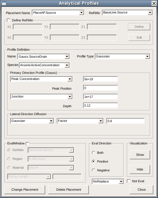

   

   Figure 3. Analytical Profiles dialog box.

2. Type PlaceAP.Source in the Placement Name field.
3. Select the baseline BaseLine.Source from the Ref/Win list.
4. Under Profile Definition, enter Gauss.SourceDrain in the Name field.
5. Select Gaussian from the Profile Type list and PhosphorusActiveConcentration from the Species list.
6. Under Primary Direction Profile (Gauss), type 5e19 in the Peak Concentration field and 0 in the Peak Position field.
7. Type 1e17 in the Junction field and 0.12 in the Depth field.
8. Under Lateral Direction Diffusion, enter 0.8 in the Factor field.
9. Click Add Placement.
10. Repeat all steps for the drain junction profile and the source/drain extensions.

Similar steps can be executed to assign the drain junction profile and the profile for the source/drain extension junctions. Use the following listed profiles accordingly.

Junction	Placement name	Baseline name	Profile name
Source	PlaceAP.Source	BaseLine.Source	Gaussian.SourceDrain
Drain	PlaceAP.Drain	BaseLine.Drain	Gaussian.SourceDrain
Source extension	PlaceAP.SourceExt	BaseLine.SourceExt	Gaussian.SourceDrainExt
Drain extension	PlaceAP.DrainExt	BaseLine.DrainExt	Gaussian.SourceDrainExt

The Gaussian profiles are defined as follows.

Profile name	Peak concentration	Peak position	Junction concentration	Junction depth	Lateral factor
Gaussian.SourceDrain	5x1019 cm-3	0 μm	1017 cm-3	0.12 μm	0.8
Gaussian.SourceDrainExt	5x1018 cm-3	0 μm	1017 cm-3	0.035 μm	0.8

The corresponding Scheme commands are:

(sdedr:define-analytical-profile-placement "PlaceAP.Source"
  "Gauss.SourceDrain" "BaseLine.Source" "Positive" "NoReplace" "Eval")

(sdedr:define-gaussian-profile "Gauss.SourceDrain"
  "ArsenicActiveConcentration" "PeakPos" 0.0 "PeakVal" 5e19
  "ValueAtDepth" 1e17 "Depth" 0.12 "Gauss" "Factor" 0.8)

(sdedr:define-analytical-profile-placement "PlaceAP.Drain"
  "Gauss.SourceDrain" "BaseLine.Drain" "Positive" "NoReplace" "Eval")

(sdedr:define-analytical-profile-placement "PlaceAP.SourceExt"
  "Gauss.SourceDrainExt" "BaseLine.SourceExt" "Positive" "NoReplace" "Eval")

(sdedr:define-gaussian-profile "Gauss.SourceDrainExt"
  "ArsenicActiveConcentration" "PeakPos" 0.0 "PeakVal" 5e18
  "ValueAtDepth" 1e17 "Depth" 0.035 "Gauss" "Factor" 0.8)

(sdedr:define-analytical-profile-placement "PlaceAP.DrainExt"
  "Gauss.SourceDrainExt" "BaseLine.DrainExt" "Positive" "NoReplace" "Eval")

The profile definition for the contact and extension profiles can be used for both the source and drain implantations.

3.4 Saving the Model

To save the model, follow the instructions in Section 2.12 Saving the Model.

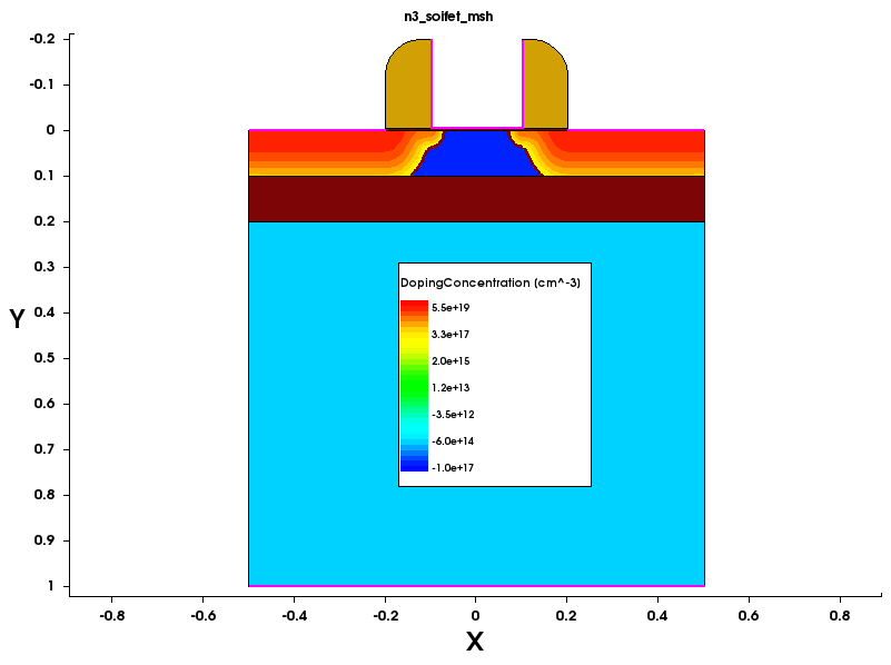
Figure 4. Device with its latest doping conditions after meshing viewed in Sentaurus Visual. (Click image for full-size view.)

Click to view all the commands discussed in this section in the command file doping_dvs.cmd.

The complete project can be investigated from within Sentaurus Workbench in the directory Applications_Library/GettingStarted/sde/soifet.

3.5 Assignment

Create the doping profile definitions for the SiGe HBT from Section 2.13 Assignment.

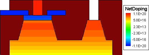
Figure 5. SiGe HBT with its latest doping conditions.

Click to view a solution of the command file sigehbt_dvs.cmd.

The complete project can be investigated from within Sentaurus Workbench in the directory Applications_Library/GettingStarted/sde/sigehbt.