
Sentaurus Device Electromagnetic Wave Solver
3. Discrete Fourier Transform
3.1 Overview
3.2 Modeling Dispersive Media
3.3 Broadband EMW Simulation Setup
3.4 Example: Broadband Simulation of Dispersive Media Using DFT
Objectives
- To understand how to model or set up dispersive media in EMW.
- To learn to use the DFT feature in broadband EMW simulations.
- To understand the limitations of DFT in EMW simulations.
3.1 Overview
For applications involving optical generation, it is often desirable to run EMW simulations over a range of wavelengths within the spectrum of interest. Rather than running multiple EMW simulations at individual wavelengths, a temporal excitation source (for example, a Gaussian pulse) can be applied during a single transient simulation.
After running this simulation, the discrete Fourier transform (DFT) can be applied to obtain the fields or other derived quantities such as optical generation, absorbed photon density, and power flux density over the range of wavelengths contained within the spectrum of interest.
This broadband approach not only simplifies the simulation or project setup, but also can reduce the total simulation time required by a significant amount compared to running a sequence of continuous wave simulations, especially when the total of number of individual wavelengths is large (> 10).
3.2 Modeling Dispersive Media
A key component of running broadband simulations in EMW is to account for the correct optical behavior (or dispersive nature) of various materials in a simulated structure over the spectrum of interest. To properly capture this behavior, the dispersive models implemented in EMW are:
- Debye
- Drude
- DrudeLorentz
- Lorentz
- SingleDipoleDebye
- SingleDipoleDrude
- ModLorentz
- DrudeModLorentz
The modified Lorentz models, ModLorentz and DrudeModLorentz, provide improved flexibility in fitting. For more details about how to create dispersive model parameters based on an existing n&k table, refer to the Sentaurus Visual module, Section 7. Special Focus: Fitting Dispersive Media for EMW.
To improve the accuracy at the interface between dispersive materials, an interface-averaging model can be activated. This implementation takes into account interfaces between dispersive media with lossy dielectrics, or interfaces between dispersive materials that are fit using the same type of dispersive model.
The interface-averaging model is activated by specifying InterfaceAveraging = yes in the DispersiveMedia section of the EMW command file. Here is an example for specifying gold as a dispersive material using the DrudeModLorentz model with interface averaging activated:
DispersiveMedia {
  Material              = { "Gold" }
  Model                 = DrudeModLorentz
  ModelParameters       = UserDefined
  deltak                = 100.0
  InterfaceAveraging    = yes
}
In this case, you must specify the fitting parameters required to fit gold over the wavelength range of interest. This is discussed in more detail in the next section.
The combined collection of dispersive models and the interface-averaging function provide users with a comprehensive capability to fit the dielectric function of a wide variety of metals, semiconductors, insulators, and other materials commonly used in EMW simulations over a specific wavelength range of interest.
For more details about the dispersive models, refer to the Sentaurus™ Device Electromagnetic Wave Solver User Guide, "Modeling of Dispersive Media".
3.3 Broadband EMW Simulation Setup
Setting up a broadband EMW simulation, in general, requires users to define or set up the following:
- Dispersive model and fitting parameters
- Broadband excitation source
- DFT wavelength table
- Plots, extractors, or sensors for DFT wavelengths
3.3.1 Specifying Dispersive Model and Defining Fitting Parameters
The dispersive material and the chosen dispersive model are both defined in the DispersiveMedia section of the EMW command file as follows:
DispersiveMedia {
  Material           = { "Aluminum" }
  Model              = DrudeModLorentz
  ModelParameters    = UserDefined
  deltak             = 100.0
  InterfaceAveraging = yes
}
In this example, aluminum is modeled as a dispersive material using the DrudeModLorentz model, and ModelParameters = UserDefined instructs EMW to set the poles for the defined model to the values specified in the user-defined pole table in the material parameter file:
Material = "Aluminum" {
  EMW {
    epsilon_r = 1.0
    sigma = 0.0
    mu_r = 1.0
    sigma_m = 0.0
    DrudeModel (
      Epsilon_inf    = 1.00000e+00
      Number_E_poles = 1
      E_polesTable (
        # frequency(Hz) damping factor(rad/s)
        3.27500e+15   2.08247e+14
      )
    )
    ModLorentzModel (
      Epsilon_static = 1.09335e+00
      Epsilon_inf = 1.00000e+00
      Number_E_poles = 5
      E_polesTable (
        # amplitude   frequency(Hz) damping factor(rad/s) damping factor'(rad/s)
        1.00000e+00 3.28219e+14   1.68960e+14           2.51043e+16
        3.74539e+01 5.87649e+14   1.70030e+15           8.59517e+09
        9.51363e+01 3.80352e+14   3.34420e+14           3.43705e+09
        1.46655e+00 3.00244e+14   4.75944e+13           3.19657e+11
        1.95679e+01 4.74851e+14   5.44254e+14           1.26736e+09
      )
    )
  }
}
In this example, aluminum was fit using the DrudeModLorentz model with six poles (one Drude pole and five modified Lorentz poles) over the range 300–1000 nm. However, if ModelParameters had been set to ComputeFromComplexRefractiveIndex, the poles for the specified dispersive model would have been extracted automatically from the CRI table values.
Setting DeltaK activates the dispersive model when k + DeltaK ≥ n, where n is the index of refraction. Setting DeltaK to a large number ensures the specified dispersive model is always activated.
3.3.2 Specifying Broadband Excitation Source
A common approach to broadband excitation is to use a Gaussian excitation source pulse, which can be defined as follows:
PlaneWaveExcitation {
  BoxCorner1  = {0.,   0.,   -0.3}
  BoxCorner2  = {0.05, 0.05, -0.3}
  Signal      = Gauss
  Delay       = 10
  Theta       = 0
  Phi         = 0
  Intensity   = 1
}
This syntax defines a normally incident (Theta=0) Gaussian pulse with an imposed Delay of 10 periods. In this case, EMW computes the width of the Gaussian pulse automatically based on the defined DFT wavelength table (discussed in the next section). TruncatedPlaneWaveExcitation also can be used if the excitation pulse must be confined to a particular spatial region of the structure.
For complete details and options for specifying temporally dependent excitations, refer to the Sentaurus™ Device Electromagnetic Wave Solver User Guide, "Temporal Dependency".
3.3.3 Setting Up the DFT Wavelength Table
The DFT section of the EMW command file is used to define the range of wavelengths over which the broadband simulation is run:
Dft {
  minWavelength       = 300
  maxWavelength       = 1000
  numberOfWavelengths = 8
}
This syntax sets up a wavelength table in 100 nm increments, which begins at 300 nm and ends at 1000 nm. The NumberOfWavelengths (Nλ) parameter determines the step size (Δλ) of the wavelength table, which is defined as Δλ = (MaxWavelength – MinWavelength)/(Nλ – 1).
3.3.4 Defining Plots, Extractors, or Sensors for DFT Wavelengths
To extract fields or derived quantities at the wavelengths specified in the DFT table, a single Plot, Extractor, or Sensor section must be defined in which those specific wavelengths of interest, or a range of wavelengths that fall within the range already established in the DFT table, are specified. This is accomplished using either the WavelengthRange or WavelengthList keyword as shown here:
Sensor {
  Name            = "total"
  Quantity        = PowerFluxDensity
  BoxCorner1      = {0.,   0.,  -0.2}
  BoxCorner2      = {0.05, 0.05,-0.2}
  Mode            = {Integrate}
  Sides           = {Zmin,Zmax}
  WavelengthList = { 300, 400, 500, 600, 700, 800, 900, 1000 }

}
Sensor {
  Name            = "reflected"
  Quantity        = PowerFluxDensity
  BoxCorner1      = {0.,   0.,   -0.4}
  BoxCorner2      = {0.05, 0.05, -0.4}
  Mode            = {Integrate}
  Sides           = {Zmin,Zmax}
  WavelengthRange = {300, 1000}

}
Sensor {
  Name            = "transmitted"
  Quantity        = PowerFluxDensity
  BoxCorner1      = {0.,   0.,   0.2}
  BoxCorner2      = {0.05, 0.05, 0.2}
  Mode            = {Integrate}
  Sides           = {Zmin,Zmax}
  WavelengthList = { 300, 400, 500, 600, 700, 800, 900, 1000 }

}
Sensor {
  Name            = "absorbed_slab"
  Quantity        = AbsorbedPowerDensity
  Region          = { "slab" }
  Mode            = {Integrate}
  WavelengthRange = {300, 1000}
}
Here, four different sensors are defined that compute the integrated power flux density ("total", "reflected", and "transmitted") and the absorbed power density ("absorbed_slab") in the "slab" region for each wavelength. The specification of either a list or a range of wavelengths is merely to demonstrate that either approach can be applied, both of which result in the integrated quantities being computed over each wavelength (that is, 300 nm, 400 nm, 500 nm, ..., 1000 nm).
When defining a specific list of wavelengths using the WavelengthList keyword, values are contained within braces. However, when specifying a range of wavelengths using the WavelengthRange keyword, the range is contained within parentheses.
3.4 Example: Broadband Simulation of Dispersive Media Using DFT
This example describes how to build a project in Sentaurus Workbench to accomplish the following:
- Build a 3D single-slab structure.
- Generate the tensor mesh.
- Set up a broadband EMW simulation for dispersive media.
- Compute and plot the power reflection coefficient versus wavelength.
Figure 1 shows the Sentaurus Workbench tool workflow for this example.
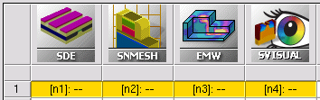
Figure 1. Workflow of Sentaurus Workbench project.
The example starts by using Sentaurus Structure Editor to build a (50 nm × 50 nm) single slab of aluminum, 80 nm thick and bounded by vacuum on the top and bottom. Figure 2 shows the resulting 3D structure.
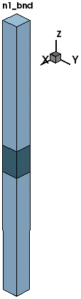
Figure 2. Three-dimensional single-slab aluminum–air structure.
Click to view the Sentaurus Structure Editor command file sde_dvs.cmd.
Next, the Sentaurus Mesh tool instance (snmesh) builds the tensor mesh. The -t -emw options are added in the Command Line field of the Tool Properties dialog box for Sentaurus Mesh (right-click the Sentaurus Mesh tool icon and select Properties) as shown in Figure 3.
These options instruct Sentaurus Mesh to build a tensor mesh and to save the resulting mesh file in TDR format. Figure 4 shows the generated tensor mesh.
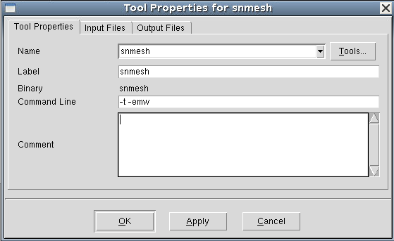
Figure 3. Tool Properties dialog box for Sentaurus Mesh tool instance.
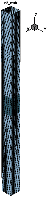
Figure 4. Tensor mesh for single-slab aluminum–air structure. (Click image for full-size view.)
Click to view the Sentaurus Mesh command file snmesh_msh.cmd.
Next, both the EMW command file and material parameter files are set up as outlined and discussed in Section 3.3 Broadband EMW Simulation Setup.
Sensors are defined in the EMW command file as illustrated in Figure 5 to capture the integrated power flux and the absorbed photon densities that are needed to compute the power reflection coefficient.
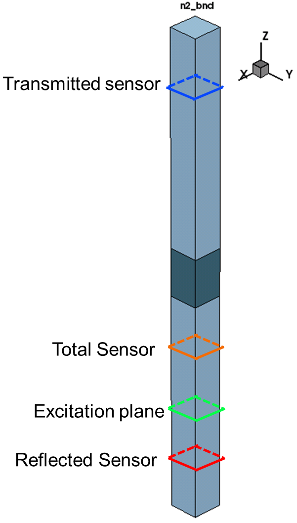
Figure 5. Location of sensors. (Click image for full-size view.)
Click to view the EMW command file emw_eml.cmd.
Click to view the material parameter file snmesh.par.
After the EMW simulation is finished, a Sentaurus Visual tool instance computes the power reflection coefficient at each DFT wavelength. Then, the results are plotted together with the analytically determined values as shown in Figure 6.
Click to view the Sentaurus Visual command file svisual_vis.tcl.
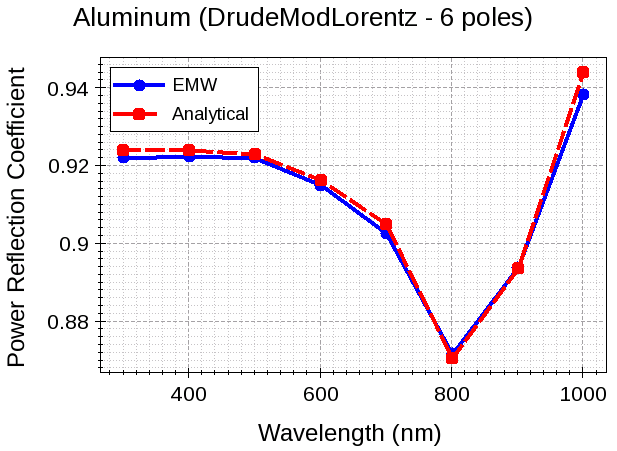
Figure 6. Plot of power reflection coefficient versus wavelength. (Click image for full-size view.)
The complete project can be investigated from within Sentaurus Workbench in the directory Applications_Library/GettingStarted/emw/3d_dispersive.
Copyright © 2017 Synopsys, Inc. All rights reserved.